
If you want to work out how much federal income tax you owe in Excel, you can’t just multiply your income by one tax rate.
The US uses progressive tax brackets. Each rate only applies to the slice of income that falls inside its bracket, not to your whole income.
So someone with $97,400 of taxable income doesn’t pay 22% on all of it.
They pay 10% on the first $12,400, 12% on the next $38,000, and 22% on the rest.
That’s why a simple lookup of “which rate applies to me” gives the wrong answer. The formula has to add up the tax from every bracket the income passes through.
In this article, I’ll show you four ways to do it: a bracket-by-bracket breakdown with helper columns, a SUMPRODUCT formula, an XLOOKUP formula, and a LET formula.
Method #1: Using Helper Columns
This is the method I’d recommend for most people. It shows exactly how much of your income lands in each bracket, so you can check every number.
Below I have the 2026 federal tax brackets for single filers on the Helper Columns sheet.
Column A has the lower limit of each bracket, column B has the upper limit, and column C has the tax rate.
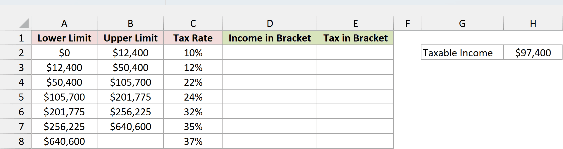
The taxable income is in cell H2 ($97,400).
I want to see how much of it falls in each bracket (column D), the tax on each slice (column E), and the total tax.
Here is the formula to enter in D2 and copy down to D8:
=MAX(0,MIN($H$2,B2)-A2)
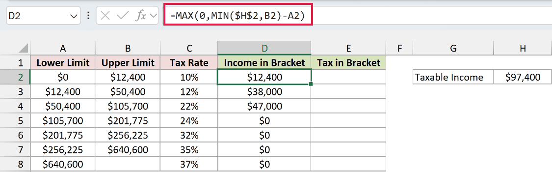
The first bracket gets $12,400, the second gets $38,000, and the third gets $47,000. That adds up to the full $97,400, and every higher bracket gets $0.
How does this formula work?
MIN($H$2,B2) returns whichever is smaller: the income or the bracket’s upper limit. So the income is capped at the top of the bracket.
Subtracting A2 (the lower limit) leaves the part of the income that sits inside that bracket.
For brackets above the income, that subtraction goes negative. MAX(0,…) turns those negative numbers into 0.
I’m copying this formula down instead of using a range, because MIN would collapse the whole range into one number.
Now let’s calculate the tax on each slice. Here is the formula to enter in E2 and copy down to E8:
=D2*C2
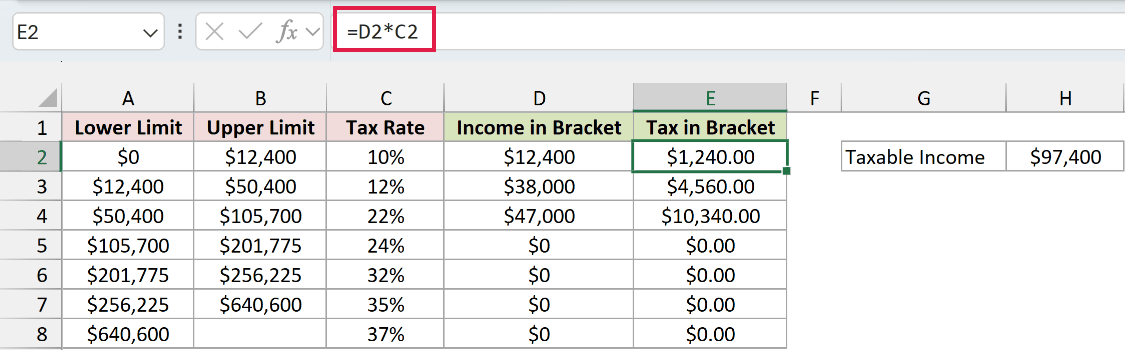
This multiplies each slice by its own rate. For example, the $38,000 in the 12% bracket returns $4,560.
Finally, here is the formula for the total tax in H3:
=SUM(E2:E8)
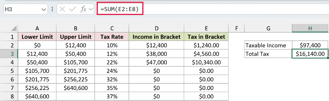
The total income tax on $97,400 is $16,140.
Note: The top bracket (37%) has no upper limit, so B8 is left blank. MIN ignores a blank cell reference, so for that row the formula uses the full income. You don’t need to type a huge number like 999,999,999 there.
Method #2: Using the SUMPRODUCT Function
If you’d rather get the tax in one cell, SUMPRODUCT can do it. It also works in every version of Excel.
Below I have the same 2026 brackets on the SUMPRODUCT sheet, and a list of employees with their taxable income in columns F and G.
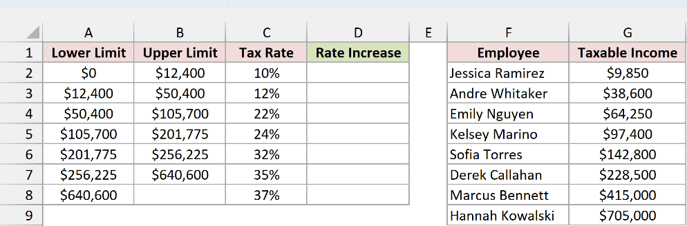
I want to calculate the income tax for each employee in column H.
This method needs one helper column in the bracket table first.
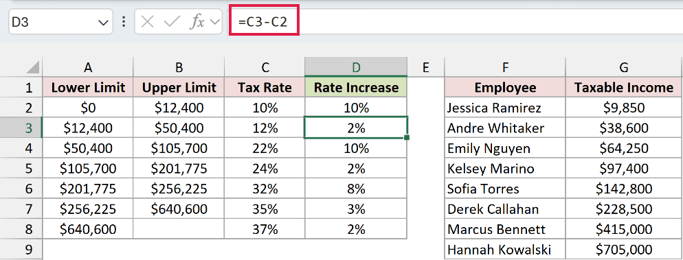
Column D holds the rate increase, which is how much each bracket’s rate goes up compared to the one below it.
In D2, enter =C2 (the first bracket has nothing below it, so its increase is the full 10%). Then enter this formula in D3 and copy it down to D8:
=C3-C2
Now here is the formula to enter in H2 and copy down to H9:
=SUMPRODUCT(--(G2>$A$2:$A$8),G2-$A$2:$A$8,$D$2:$D$8)
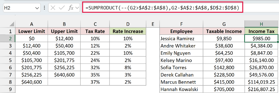
Kelsey Marino has $97,400 of taxable income, and the formula returns $16,140. That’s the same answer as Method #1.
How does this formula work?
The trick here is to think of the tax in layers. Every dollar above $0 is taxed at 10%.
Every dollar above $12,400 gets an extra 2%, every dollar above $50,400 an extra 10%, and so on.
–(G2>$A$2:$A$8) returns 1 for each bracket the income has reached and 0 for the rest. For $97,400, only the first three brackets get a 1.
G2-$A$2:$A$8 returns how far the income goes past each lower limit.
SUMPRODUCT multiplies those three arrays together and adds up the result. For Kelsey, that’s $9,740 + $1,700 + $4,700, which is $16,140.
The formula works out one person’s tax, so I copy it down for each employee.
Note: The rate increase column updates itself when you change the rates in column C. But if you add or remove a bracket, extend all three ranges in the formula to match.
Method #3: Using the XLOOKUP Function
This method follows the way the IRS lays out its own tax rate schedules: a fixed amount of tax, plus a percentage of the income above the bracket’s lower limit.
Below I have the 2026 brackets on the XLOOKUP sheet, along with the same employees and their taxable income in columns F and G.
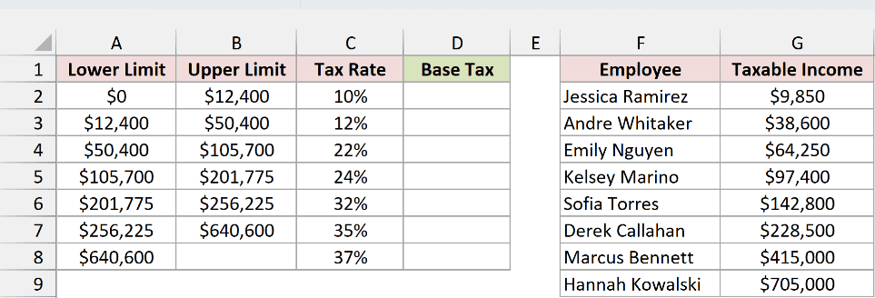
I want the income tax for each employee in column H.
First, I need a Base Tax column. It holds the total tax on all the brackets below the current one.
In D2, enter 0, since nothing sits below the first bracket. Then enter this formula in D3 and copy it down to D8:
=D2+(B2-A2)*C2
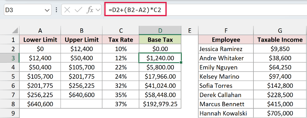
Each row takes the base tax from the row above and adds the tax on that full bracket.
For the 22% bracket, the base tax is $5,800 ($1,240 from the 10% bracket plus $4,560 from the 12% bracket).
Now here is the formula to enter in H2:
=XLOOKUP(G2:G9,A2:A8,D2:D8,,-1)+(G2:G9-XLOOKUP(G2:G9,A2:A8,A2:A8,,-1))*XLOOKUP(G2:G9,A2:A8,C2:C8,,-1)
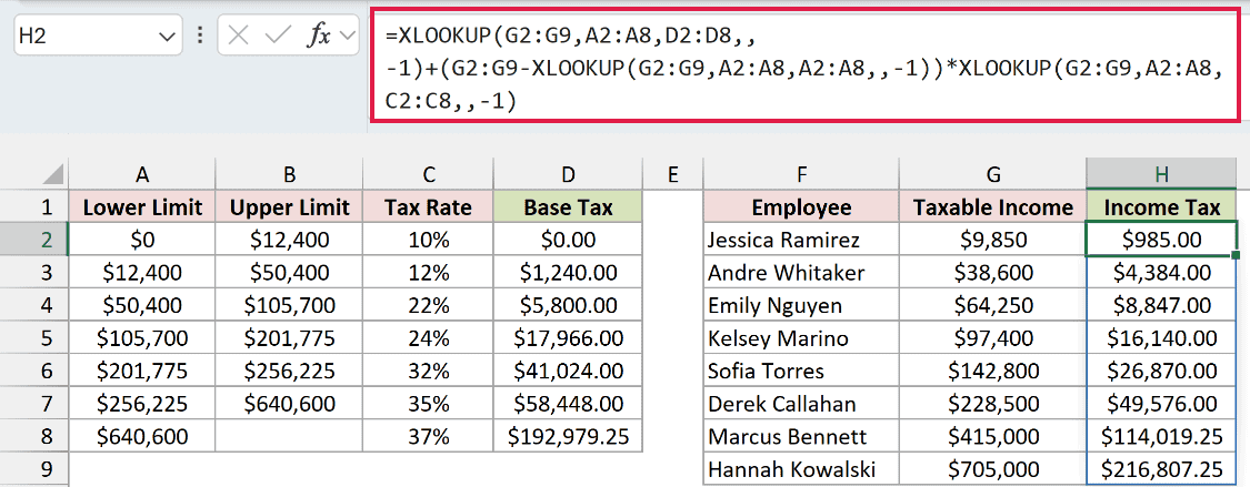
The formula spills down the column automatically and returns the tax for all eight employees.
How does this formula work?
All three XLOOKUP functions use -1 as the last argument.
That tells XLOOKUP to find an exact match or the next smaller value, so each income lands in its own bracket.
The first XLOOKUP returns the base tax for that bracket. For Kelsey’s $97,400, that’s $5,800.
The second XLOOKUP returns the bracket’s lower limit ($50,400). Subtracting it from the income gives $47,000, the part taxed at the bracket’s own rate.
The third XLOOKUP returns that rate (22%). So the formula works out $5,800 + $47,000 × 22%, which is $16,140.
Note: XLOOKUP is available in Excel 2021, Excel 2024, and Microsoft 365. In older versions, VLOOKUP with an approximate match does the same job. Enter =VLOOKUP(G2,$A$2:$D$8,4,TRUE)+(G2-VLOOKUP(G2,$A$2:$D$8,1,TRUE))*VLOOKUP(G2,$A$2:$D$8,3,TRUE) in H2 and copy it down.
Method #4: Using the LET Function
If you have Excel 2021 or later (including Microsoft 365), you can skip the helper columns completely.
LET lets you name each part of the calculation inside one formula, which keeps it readable.
Below I have the 2026 brackets on the LET Formula sheet, with the employees and their taxable income in columns E and F.
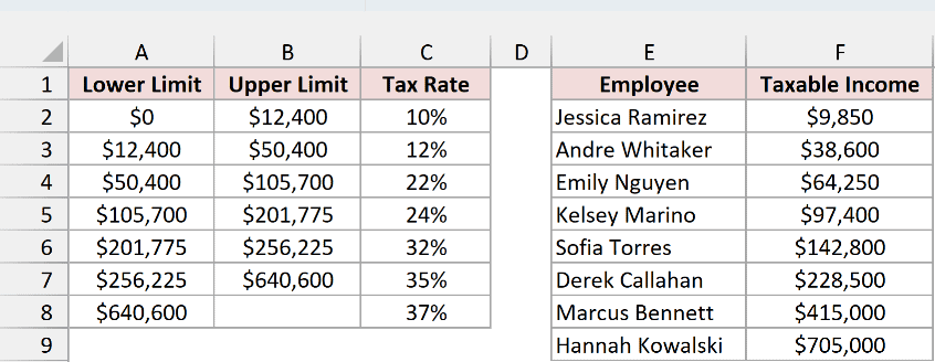
I want the income tax for each employee in column G, using only the three columns of the bracket table.
Here is the formula to enter in G2 and copy down to G9:
=LET(income,F2,lower,$A$2:$A$8,upper,$B$2:$B$8,rate,$C$2:$C$8,top,IF(upper="",income,upper),slice,IF(income<top,income,top)-lower,SUM(IF(slice>0,slice,0)*rate))
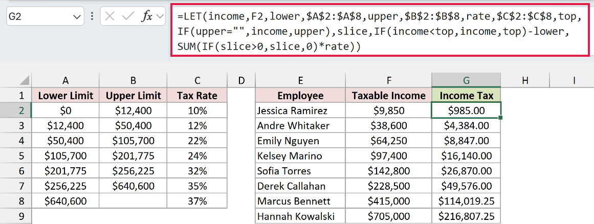
Hannah Kowalski has $705,000 of taxable income, which reaches the 37% bracket. The formula returns $216,807.25.
How does this formula work?
This is Method #1 squeezed into a single cell. The first four names (income, lower, upper, and rate) point to the income cell and the three bracket columns.
top replaces the blank upper limit of the last bracket with the income itself. That way, the 37% bracket has a ceiling to work with.
slice caps the income at each bracket’s upper limit and subtracts the lower limit. It returns the amount in each bracket, with negative numbers for brackets the income never reaches.
The last line turns those negatives into 0, multiplies each slice by its rate, and adds everything up with SUM.
The SUM at the end returns one total per person, so I copy the formula down instead of spilling it.
Finding the Effective and Marginal Tax Rate
Once you have the total tax, two more numbers are worth knowing.
The effective tax rate is the share of your income that goes to tax. The marginal tax rate is the rate on your last dollar.
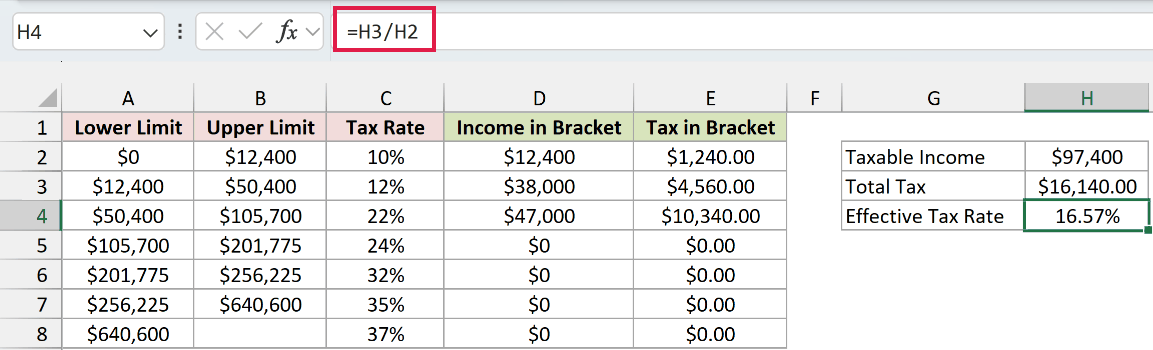
Back on the Helper Columns sheet, the taxable income is in H2 and the total tax is in H3.
Here is the formula for the effective tax rate in H4:
=H3/H2
And here is the formula for the marginal tax rate in H5:
=XLOOKUP(H2,A2:A8,C2:C8,,-1)
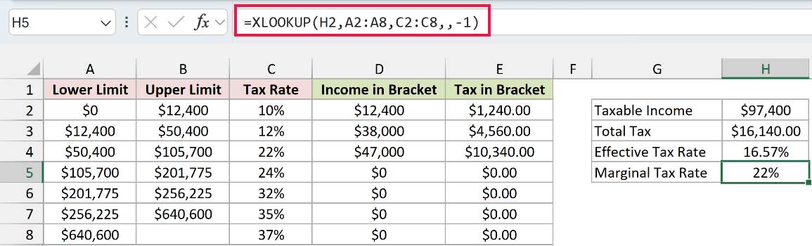
On $97,400, the effective rate is 16.57% and the marginal rate is 22%. That gap is why multiplying the whole income by 22% overstates the tax.
Additional Notes About Calculating Income Tax in Excel
- Use taxable income, not gross income. The brackets apply after deductions. For 2026, the standard deduction is $16,100 for single filers and $32,200 for married couples filing jointly.
- Married couples filing jointly have different brackets. For 2026, the limits are $24,800, $100,800, $211,400, $403,550, $512,450, and $768,700. Swap them into the table, keep the same rates, and every formula keeps working.
- Your tax return may be off by a few dollars. If your taxable income is under $100,000, Form 1040 uses the IRS Tax Table, which taxes small income ranges (mostly $50 wide). These formulas calculate the exact amount.
- These formulas cover federal income tax only. State income tax, Social Security, and Medicare are calculated separately and aren’t included here.
Frequently Asked Questions
Here are some questions people often ask about working out income tax in Excel.
Does moving into a higher tax bracket mean all my income is taxed at the higher rate?
No. Only the income above the bracket’s lower limit is taxed at the higher rate.
Everything below it is still taxed at the lower rates, which is what all four methods above calculate.
Why not just use a nested IF formula?
You can use nested IFs, but you have to type every threshold and every running total into the formula itself.
When the brackets change next year, you have to rewrite it. With a bracket table, you only update the table.
How do I update the formulas for a new tax year?
Replace the lower limits, upper limits, and rates in the bracket table with the new figures from the IRS. The helper columns and formulas recalculate on their own.
Can I use these formulas for another country’s tax brackets?
Yes, as long as the tax is progressive (each rate applies only to its own band of income).
Enter that country’s thresholds and rates in the bracket table, and the formulas work the same way.
Conclusion
In this article, I showed you four ways to calculate income tax in Excel using tax brackets: helper columns, SUMPRODUCT, XLOOKUP, and LET.
For most people, the helper columns in Method #1 are the easiest to follow and check.
I hope you found this article helpful.
Other Excel articles you may also like:
