How to Paste into Filtered Column Skipping the Hidden Cells?

Copying and pasting are probably one of the most used actions in an Excel spreadsheet.

But when it comes to filtered data, copy-pasting data is not always smooth.

Ever tried pasting something to a table that has been filtered? It’s not as easy as it sounds.

In this tutorial, I will show you how to copy data from a filtered dataset and how to paste in a filtered column while skipping the hidden cells.

Copying from a Filtered Column Skipping the Hidden Cells

Suppose you have the below dataset:

Given the above table, say you want to copy all the rows of employees from the IT department only.

For this, you can apply a filter to your table as follows:

1. Select the entire table.
2. From the Data tab, select the ‘Filter’ button under the ‘Sort & Filter’ group.
3. You will notice small arrows on every cell of the header row. These are meant to help you filter your cells. You can click on any arrow to choose a filter for the corresponding column.
4. In this example, we want to filter out only the rows that contain the Department “IT”. So, select the arrow next to the Department header and uncheck the boxes next to all the departments, except “IT”. You can simply uncheck “Select All” to quickly uncheck everything and then just select “IT”.
5. Click OK. You will now see only the rows with Department “IT”.

Now, copying from a filtered table is quite straightforward. When you copy from a filtered column or table, Excel automatically copies only the visible rows.

So, all you need to do is:

1. Select the visible rows that you want to copy.
2. Press CTRL+C or right-click->Copy to copy these selected rows.
3. Select the first cell where you want to paste the copied cells.
4. Press CTRL+V or right-click->Paste to paste the cells.

This should cause only the visible rows from the filtered table to get pasted.

Occasionally you might come across issues in copying the visible rows, especially when working with Subtotals or similar features.

In such cases, copying only the visible rows is quite easy too. Here’s what you need to do:

1. Select the visible rows that you want to copy.
2. Press ALT+; (ALT key and semicolon key together). If you’re on a Mac, press Cmd+Shift+Z. This shortcut lets you select only the visible rows, while skipping the hidden cells.
3. Press CTRL+C or right-click->Copy to copy these selected rows.
4. Select the first cell where you want to paste the copied cells.
5. Press CTRL+V or right-click->Paste to paste the cells.

So you see copying from filtered columns is quite straightforward.

But you can’t say the same when it comes to pasting to a filtered column.

Also read: How to Delete Filtered Rows in Excel (with and without VBA)

Pasting a Single Cell Value to All the Visible Rows of a Filtered Column

When it comes to pasting to a filtered column, there may be two cases:

• You might want to paste a single value to all the visible cells of the filtered column.
• You might want to paste a set of values to visible cells of the filtered column.

For the first case, pasting into a filtered column is quite easy.

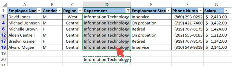
Let’s say we want to replace all the cells that have Department = “IT” with the full form: “Information Technology”.

For this, you can type the word “Information Technology” in any blank cell, copy it, and paste it to the visible cells of the filtered “Department” Column. Here’s a step-by-step on how to do this:

1. Select a blank cell and type the words “Information Technology”.
2. Copy it by press CTRL+C or Right click->Copy.
3. Select all the visible cells in the column with the “Department” header.
4. Paste the copied value by pressing CTRL+V or Right click->Paste.

You will find the value “Information Technology” pasted to only the visible cells of the column “Department”.

To verify this, remove the filter by selecting the Data->Filter. Notice that all the other cells of the “Department” column remain unchanged.

Also read: How to Filter as You Type in Excel

Two Ways to Paste a Set of Values to Visible Rows of a Filtered Column

Now let’s see what happens when you want to paste a set of values to the visible cells of a filtered column. Say you want to paste a list of salaries for only the rows containing Department=”Information Technology”.

If you try copying these cells and pasting them to the filtered Salary column, you will probably get an error message like “The command cannot be used on multiple selections”.

This is because you cannot paste to cells in a range that contains hidden rows or columns. It’s one of Excel’s limitations. There’s no way around that, but there are some tricks that you can use to get this done.

Here are two tricks that you can use to paste a set of values to a filtered column, skipping the hidden cells.

Pasting a Set of Values to Visible Rows of a Filtered Column – Using a Formula

In this method, we use a formula to simply copy the value of the cell to the destination cell.

For the above example (where you want to copy a set of salary values to only the rows of with Department= “Information Technology”), here are the steps you need to follow:

1. Press the equal sign (‘=’) in the first cell of the column you want to paste to (G3).
2. Now select the first cell from the list you want to copy (H3 in our example).
3. This will just create a reference to the cell. You should see the formula: =H3 in cell G3.
4. Copy this formula down by dragging down the fill handle (at the bottom right corner of cell G3). This should paste the formula only to the visible cells of column G.
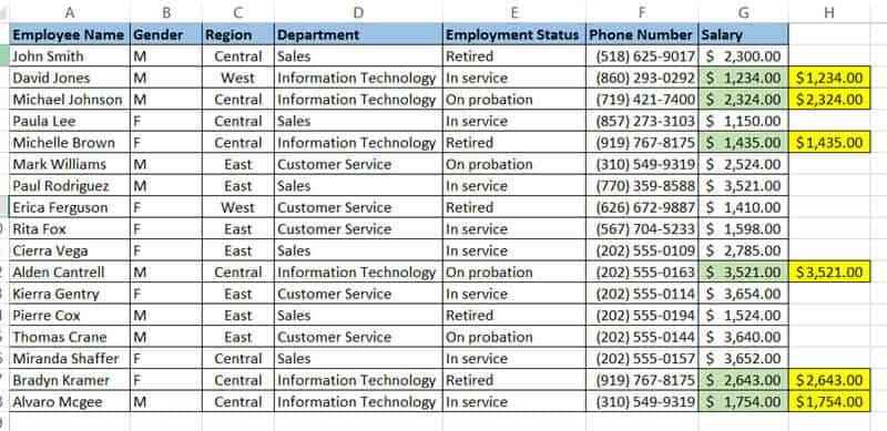
5. To verify this, remove the filter by selecting Data->Filters. Here’s an image of column G without filters after the copy-paste operation. To make it clearer for you to see, I’ve highlighted the copied cells in light green.
6. Now what you copied were just references to the original cells. So if you try to remove the original cells once you’re done copy-pasting, the copied values will disappear from column G too.
7. To avoid this, you need to paste these formula results as values. This is quite easy. While you’re in the unfiltered mode, copy all the cells of column G, right-click and select ‘Paste Values’ from the popup menu.
8. That’s it, you can now go ahead and delete the original values.

Pasting a Set of Values to Visible Rows of a Filtered Column – Using VB Script

This is a fairly easier and quicker method. All you need to do is copy the VBScript given below into your developer window and run it.

'Code developed by Steve Scott from https://spreadsheetplanet.com
Sub paste_to_filtered_col()
Dim s As Range
Dim visible_source_cells As Range
Dim destination_cells As Range
Dim source_cell As Range
Dim dest_cell As Range

Set s = Application.Selection

s.SpecialCells(xlCellTypeVisible).Select

Set visible_source_cells = Application.Selection
Set destination_cells = Application.InputBox("Please select the destination cells:", Type:=8)

For Each source_cell In visible_source_cells
    source_cell.Copy
    For Each dest_cell In destination_cells
        If dest_cell.EntireRow.RowHeight <> 0 Then
            dest_cell.PasteSpecial
            Set destination_cells = dest_cell.Offset(1).Resize(destination_cells.Rows.Count)
            Exit For
        End If
    Next dest_cell
Next source_cell

End Sub

Here are the steps to put this code in your Excel workbook so that you can use it:

1. Select all the rows you need to filter (including the column headers).
2. From the Developer Menu Ribbon, select Visual Basic.
3. Once your VBA window opens, Click Insert->Module and paste the above code into the module window.

Your macro is now ready to run.

Here are the steps to run the code to paste in a filtered column while skipping the hidden cells:

1. First, select the cells that you want to copy.
2. Run the script by navigating to Developer tab, clicking on the Macros option, and then the select the paste_to_filtered_col macro in the Macro dialog box
3. The code will ask you to select your destination cells (where you want to paste the copied cells).
4. Select the cells and click OK.

Your selected cells will now be copied and pasted to the destination cells. You can go ahead and delete the original cells if you want.

By the end of this, you will have copied each visible cell from the source range to the destination range, skipping any hidden rows in the destination.

Explanation of the VBA code:

Variable Declarations:

• Dim s As Range: Declares s as a range object, which will later hold the cells selected by the user.
• Dim visible_source_cells As Range, destination_cells As Range: Declares visible_source_cells to hold the cells that are visible, and destination_cells to hold the cells where the content will be pasted.
• Dim source_cell As Range, dest_cell As Range: Declares two more range objects, source_cell, and dest_cell, which will represent individual cells in the source and destination ranges, respectively.

VBA Code Explanation:

• Set s = Application.Selection: This line sets the variable ‘s’ to the currently selected range in the worksheet.
• s.SpecialCells(xlCellTypeVisible).Select: This line only selects the visible cells from the range s (which are the selected range of cells).
• Set visible_source_cells = Application.Selection: Assigns the selected (visible) cells to the variable visible_source_cells.
• Set destination_cells = Application.InputBox(“Please select the destination cells:”, Type:=8): This line prompts the user to select the destination cells and then stores that cell reference in the destination_cells variable.
• For Each source_cell In visible_source_cells: This starts a For Each loop that goes through each visible cell in the source range.
  • source_cell.Copy: This line copies the current source_cell.
  • For Each dest_cell In destination_cells: This starts another For Each loop that iterates through each cell in the destination range.
    • If dest_cell.EntireRow.RowHeight <> 0 Then: This checks if the row height of the dest_cell is not equal to 0. If this condition is True, that means that the destination cell is not hidden.
      • dest_cell.PasteSpecial: Pastes the copied cell’s content into dest_cell (as it’s not hidden)
      • Set destination_cells = dest_cell.Offset(1).Resize(destination_cells.Rows.Count): Resizes and shifts the destination_cells range down by one.
    • Exit For: Exits the inner loop after the first visible dest_cell is found and pasted into.
• Next source_cell: Goes back to step 5 to process the next source_cell.

Note: One important thing to keep in mind when using the VBA code is that the change is done by the code cannot be undone. So it’s strongly advisable that you create a backup copy of your work before using the vba code.

Adding the Macro to Quick Access Toolbar

You can also create a small shortcut (using the Quick Access Toolbar) to run your macro whenever you need it.

Here’s are the steps to do this:

1. Click the Customize Toolbar arrow, which you’ll find above Excel’s menu ribbon.
2. Select ‘More Commands’ from the dropdown menu that appears.
3. This will open the ‘Excel Options’ dialog box.
4. Click on the drop-down list below ‘Choose Commands From’ and select ‘Macros’.
5. Select the name of the macro you created. In our case, it’s ‘ThisWorkbook.paste_to_filtered_col’ Click on the ‘Add>>’ button.
6. Click OK.

You’ll now get a Quick Access macro button to quickly run your macro with a single click.

Whenever you need to copy and paste a set of cells to a filtered column, just select your source cells, click on this created button and then select the destination cells.

When you click OK, you should get your source cells copied into your selected destination cells.

So this is how you can copy and paste in a filtered column while skipping the cells in the hidden rows.

I hope you found this tutorial useful!

Other Excel tutorials you may like:

• How to Unsort in Excel (Revert Back to Original Data)
• How to Hide Rows based on Cell Value in Excel
• How to Compare Two Cells in Excel?
• How to Paste without Formatting in Excel (Shortcuts)
• How to Clear Filter in Excel? Shortcut!
• Copy and Paste shortcuts in Excel
• How to Filter by Color in Excel?