Excel provides features such as filters that let you hide rows based on cell values. However, if you want to hide columns based on cell values, there’s, unfortunately, no dedicated ‘feature’ or menu item for that.
That’s not to say that it’s not possible to hide columns in Excel based on cell values. You only need to take a little more effort to do that.
Enter Excel macros and VBA!
Excel macros along with VBA provide excellent tools that let you do just about anything you want to do with your Excel sheets. That includes hiding or un-hiding columns depending on values in certain cells.
In this tutorial, we will see how you can use Excel VBA to hide columns based on cell values.
We will first look at an example where changes take place only when you run a macro. After that, we will look at another example where the changes take place in real-time, whenever the value of a cell changes.
Hiding Columns Based on Cell Value when Macro is Executed
In this example, we will show you how to hide all columns that contain a particular value in a given cell.
The value, based on which you want to hide the columns, can be anything you like. It can be a number, a letter, a word, or even a phrase.
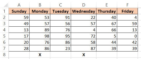
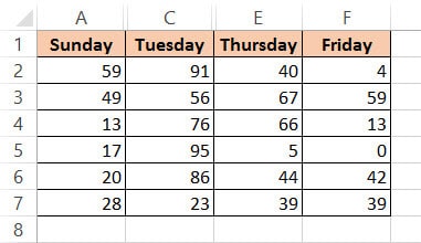
Let us use the following dataset to demonstrate:

Say you have columns containing sales figures for Monday through Friday, and you want to run a macro to hide all columns that have the letter X in row 8.
For this, we need a macro that will loop through each cell of row 8 and hide the corresponding column.
It should essentially analyze each cell from A8 to F8 and adjust the ‘Hidden’ attribute of the column that you want to hide.
Writing the VBA Code
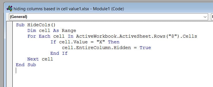
Here’s the code we used:
Sub HideCols()
Dim cell As Range
For Each cell In ActiveWorkbook.ActiveSheet.Rows("8").Cells
If cell.Value = "X" Then
cell.EntireColumn.Hidden = True
End If
Next cell
End SubTo enter the above code, all you have to do is copy it and paste it in your developer window. Here’s how:
- From the Developer menu ribbon, select Visual Basic
- Once your VBA window opens, you will see all your project files and folders in the Project Explorer on the left side. If you don’t see the Project Explorer, click on View->Project Explorer
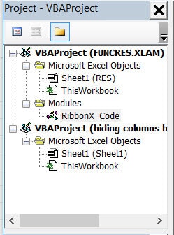
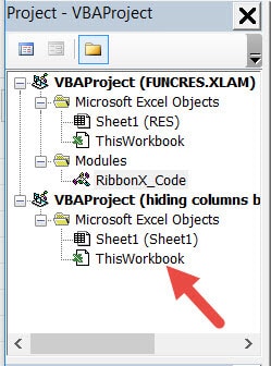
- Make sure ‘ThisWorkbook’ is selected under the VBA project with the same name as your Excel workbook.
- Click Insert->Module. You should see a new module window open up.
- Now you can start coding. Copy the above lines of code and paste them into the new module window.
- In our example, we want to hide the columns that contain an ‘X’ in row 8. But you can replace the row number from “8” in line 3 to the row number that you plan to put your ‘X’s in.
- Close the VBA window.
Note: If you can’t see the Developer ribbon, from the File menu, go to Options. Select Customize Ribbon and check the Developer option from Main Tabs. Finally, click OK.
Running the Macro
That’s it, your macro is ready to use. Now whenever you need to use it, you simply need to run it. Here’s how:
- Put X’s in row 8 for all the rows that you want to hide. We want to hide columns for Monday and Wednesdays (Columns B and D), so we added an X in cells B8 and D8.
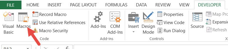
- Select the Developer tab
- Click on the Macros button (under the Code group).
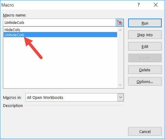
- This will open the Macro Window, where you will find the names of all the macros that you have created so far.
- Select the macro (or module) named ‘HideCols’ and click on the Run button.

- You should see all the columns marked with an X in row 8 hidden (columns B and D).
Explanation of the Code
Let us take a few minutes to understand this code
- In line 1 we defined the function name.
Sub HideCols()- In line 2 we defined a variable called cell, which can refer to a range of cells.
Dim cell As Range- In lines 3 to 7, we looped through each cell in row “8” of the Active Worksheet. If the cell contains the value “X”, then we set the ‘Hidden’ attribute of the entire column (corresponding to that cell) to True, which means we want to hide the entire corresponding column.
For Each cell In ActiveWorkbook.ActiveSheet.Rows("8").Cells
If cell.Value = "X" Then
cell.EntireColumn.Hidden = True
End If
Next cell- Line 8 simply demarcates the end of the HideCols sub-routine
End SubIn this way, the above code hides all the columns containing an ‘X’ in row 8.
Also read: Change Cell Color Based on Value of Another Cell in Excel
Un-hiding Columns Based on Cell Value when Macro is Executed
Now what do we do if we want to see the hidden rows again?
It’s quite simple. All you need to do is make a small change to the HideCols function. Repeat the same steps as above to create a new macro. Copy and paste the following code into it:
Sub UnhideCols()
Dim cell As Range
For Each cell In ActiveWorkbook.ActiveSheet.Rows("8").Cells
If cell.Value = "X" Then
cell.EntireColumn.Hidden = False
End If
Next cell
End SubNotice all we did is change line 5 from:
cell.EntireColumn.Hidden = True
to:
cell.EntireColumn.Hidden = False
In other words, we set the ‘Hidden’ attribute for the column to False, because we want Excel to unhide (or display) the corresponding columns containing an ‘X’ in row 8.
You can run this macro in exactly the same way as HideCols.
Hiding Columns in Real-time Based on a Cell Value
In the first example, the columns are hidden only when the macro runs. However, most of the time, we want to hide columns on-the-fly, based on the value in a particular cell.
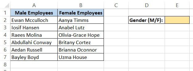
So, let’s now take a look at another example that demonstrates this. In this example, we have the following dataset:
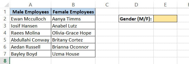
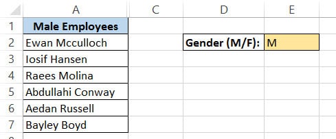
In the above dataset, we have a list of male and female employee names in two separate columns (A and B). We want only the male employee names to be displayed when cell E2 contains the value “M”. In other words, we want to hide the names of female employees.
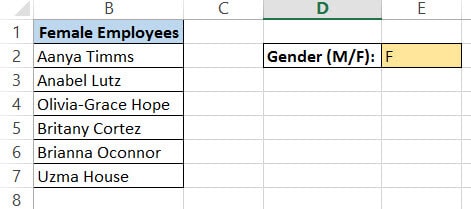
Similarly, we want only the female employee names to be displayed when cell E2 contains the value “F”. In other words, we want to hide the names of the male employees when that happens.
When there is nothing in cell E2, we want both male and female employee names to be displayed.
We want this to happen in real-time, every time the value in cell E2 changes. For this, we need to make use of Excel’s Worksheet_SelectionChange function.
The Worksheet_SelectionChange Function
The Worksheet_SelectionChange procedure is an Excel built-in function and comes pre-installed with the worksheet. It is called whenever a user selects a cell and then changes his/her selection to some other cell.
Since this function comes pre-installed with the worksheet, you need to place it in the code module of the right sheet so that you can use it. In our code, we are going to put all our lines inside this function, so that they get executed whenever the user changes the value in E2 and then selects something else.
Writing the VBA Code
Here’s the code we used:
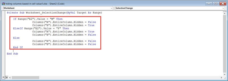
Private Sub Worksheet_SelectionChange(ByVal Target As Range)
If Range("E2").Value = "M" Then
Columns("A").EntireColumn.Hidden = False
Columns("B").EntireColumn.Hidden = True
ElseIf Range("E2").Value = "F" Then
Columns("A").EntireColumn.Hidden = True
Columns("B").EntireColumn.Hidden = False
Else
Columns("A").EntireColumn.Hidden = False
Columns("B").EntireColumn.Hidden = False
End If
End SubTo enter the above code, all you have to do is copy it and paste it in your developer window, inside your worksheet’s Worksheet_SelectionChange procedure. Here’s how:
- From the Developer menu ribbon, select Visual Basic.
- Once your VBA window opens, you will see all your project files and folders in the Project Explorer on the left side.
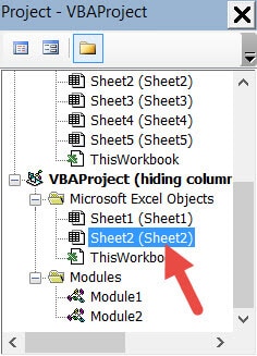
- In the Project Explorer, double click on the name of your worksheet, under the VBA project with the same name as your Excel workbook. In our example, we are working with Sheet2.
- This will open up a new module window for your selected sheet.
- Copy the above lines of code and paste them into the code window
- In our example, we want to hide column A when cell E2 contains the value ‘M’. You can replace the column name ‘A’ (in lines 3, 6, and 9) with the name of the column you want to hide.
- Similarly, we want to hide column B when cell E2 contains the value ‘F’. You can replace the column name ‘B’ (in lines 4, 7, and 10) with the name of the column you want to hide.
- You can also change the values ‘M’ and ‘F’ in lines 2 and 5 with the values you need.
- You can change the cell reference “E2” in lines 2 and 5 to references to the cell containing your deciding value.
- Close the VBA window.
Running the Macro
The Worksheet_SelectionChange procedure starts running as soon as you are done coding. So you don’t need to explicitly run the macro for it to start working.
Try typing the letter ‘M’ in capitals in the cell E2, then clicking any other cell. You should find column B (containing female employee names) disappear.
Now try typing the letter ‘F’ in capitals in cell E2, then clicking any other cell. You should find column A (containing male employee names) disappear and column A (containing female employee names) appear.
Now try removing the value in cell E2 and leaving it empty. Then click on any other cell. You should find both columns A and B become visible again.
This means the code is working in real-time as when changes are made to cell E2.
Explanation of the Code
Let us take a few minutes to understand this code now.
- Line 1 contains the header for the Worksheet_SelectionChange procedure. Notice we passed a parameter, Target to this procedure, which is of the data type Range. This parameter refers to the SelectionChange Range, and it can consist of one or more cells.
Private Sub Worksheet_SelectionChange(ByVal Target As Range)- Lines 2 to 4 check if the value in cell E2 equals ‘M’. If it does, then column B is hidden and column A is displayed. If cell E2 does not contain the value ‘M’, then control goes to line 5.
If Range("E2").Value = "M" Then
Columns("A").EntireColumn.Hidden = False
Columns("B").EntireColumn.Hidden = True
- Lines 5 to 7 check if the value in cell E2 equals ‘F’. If it does, then column A is hidden and column B is displayed. If cell E2 contains neither values ‘F’ nor ‘M’, then control goes to line 8.
ElseIf Range("E2").Value = "F" Then
Columns("A").EntireColumn.Hidden = True
Columns("B").EntireColumn.Hidden = False
- Lines 8 to 10 are executed if cell E2 contains neither ‘F’ nor ‘M’. That means if cell E2 is empty, then lines 8 to 10 are executed. Thus, both columns A and B are made visible.
Else
Columns("A").EntireColumn.Hidden = False
Columns("B").EntireColumn.Hidden = False
In this way, the above code hides column B (while column A is displayed) when cell E2 contains the value ‘M’. It hides column A (while column B is displayed) when cell E2 contains the value ‘F’.
If E2 does not contain any value then the code displays both columns A and B!
In this tutorial, we showed you how you can use Excel VBA to hide columns based on a cell value.
We did this with the help of two simple examples – one that removes required columns only when the macro is explicitly run and another that works in real-time.
We hope that we have been successful in helping you understand the concept behind the VBA macro code so that you can customize it and use it in your own applications. Happy coding!
Other Excel tutorials you may like:
- How to Hide Rows based on Cell Value in Excel
- How to Delete Hidden Rows or Columns in Excel?
- How to Unhide All Rows in Excel with VBA
- How to Remove Macros from Excel?
- How to Delete Filtered Rows in Excel (with and without VBA)
- How to Filter as You Type in Excel (With and Without VBA)
- How to Delete a Sheet in Excel Using VBA
- How to Move Row to Another Sheet Based On Cell Value in Excel?
Dear Steve,
Thank you for the vba code to hide and unhide columns based on cell data. That was exactly the code i was looking for. The reason for this post is to ask how I would go about linking both those bits of code to a single macro button so the user can hide and then unhide the columns by just clicking the one button?