
The ADDRESS function in Excel returns a cell address as text from a row number and column number.
You can choose absolute or relative notation and include a sheet name. The result is text; use INDIRECT if a formula needs to treat it as a reference.
In this article, I’ll show you how to build cell and range addresses, switch reference styles, and retrieve a value from a generated address.
ADDRESS Function Syntax in Excel
The ADDRESS function uses the following syntax:
=ADDRESS(row_num, column_num, [abs_num], [a1], [sheet_text])
row_numis the required row number.column_numis the required column number.abs_numis optional. It controls whether the row and column are absolute, relative, or mixed.a1is optional. Use TRUE or omit it for A1 notation. Use FALSE for R1C1 notation.sheet_textis optional. It adds a worksheet name to the address.
ADDRESS returns text, not a live reference. If you need a broader introduction to that distinction, see how to get a cell address instead of its value.
When to Use ADDRESS Function
- Create cell addresses from calculated row and column numbers.
- Generate absolute, relative, or mixed reference text.
- Build addresses in either A1 or R1C1 notation.
- Add sheet names to addresses used in reports or instructions.
- Assemble range text from separate start and end coordinates.
Example 1: Create Relative Cell Addresses from Row and Column Numbers
Let’s start with a warehouse checkpoint list. Each checkpoint has a row number and a column number.
Below is the dataset with an empty Relative Address column.
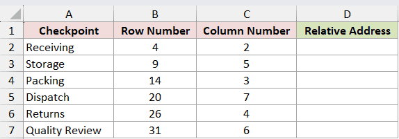
I want to return a relative A1-style address for every checkpoint with one formula.
Here is the formula:
=ADDRESS(B2:B7,C2:C7,4)
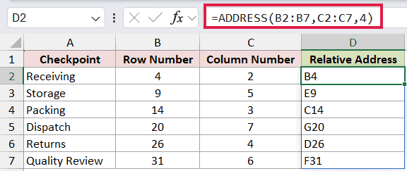
The third argument is 4, so Excel leaves both the row and column relative. The formula spills B4, E9, C14, G20, D26, and F31 into D2:D7.
You can often calculate the inputs with the ROW function or COLUMN function. Here, the row and column numbers are already listed in the table.
Example 2: Control Absolute and Relative References
The abs_num argument lets you choose where dollar signs appear.
Below is a parameter card with row 18 and column 6.
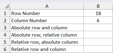
I want to generate all four possible reference types for cell F18.
For an absolute row and absolute column, use:
=ADDRESS(B1,B2,1)
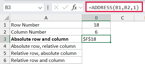
This returns $F$18.
For an absolute row and relative column, use:
=ADDRESS(B1,B2,2)
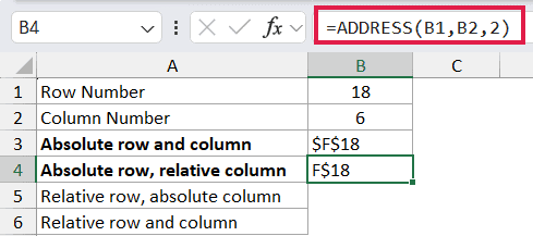
This returns F$18.
For a relative row and absolute column, use:
=ADDRESS(B1,B2,3)
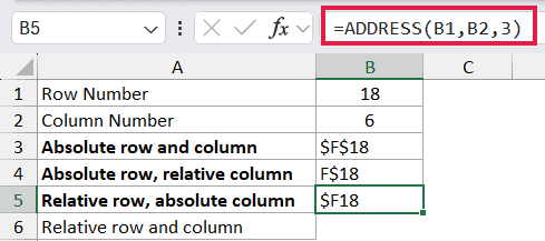
This returns $F18.
For a relative row and relative column, use:
=ADDRESS(B1,B2,4)
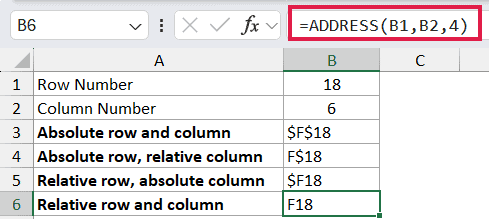
This returns F18.
The dollar signs have the same meaning as they do in an ordinary formula. Our guide to absolute cell references explains how each style behaves when copied.
Pro Tip: Remember the pattern 1, 2, 3, 4. One fixes everything, two fixes the row, three fixes the column, and four fixes nothing.
Example 3: Switch Between A1 and R1C1 Reference Styles
ADDRESS can return the same location in either A1 or R1C1 notation.
Below is a parameter card with row 12 and column 7.
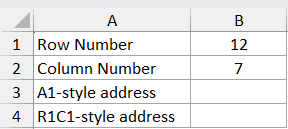
To return the address in A1 notation, use TRUE for the fourth argument:
=ADDRESS(B1,B2,1,TRUE)
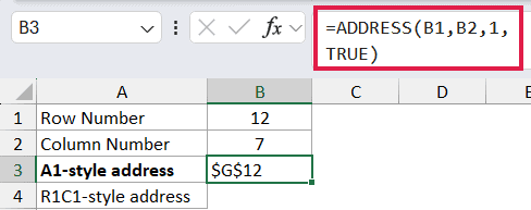
The formula returns $G$12.
To return the same location in R1C1 notation, use FALSE:
=ADDRESS(B1,B2,1,FALSE)
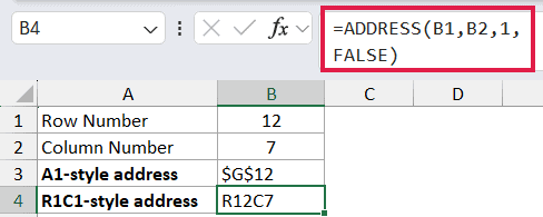
This returns R12C7. The R identifies the row, and the C identifies the column.
Example 4: Add Sheet Names to Cell Addresses
The optional sheet_text argument qualifies an address with a worksheet name.
Below is a list of report sections with their sheet names, row numbers, and column numbers.
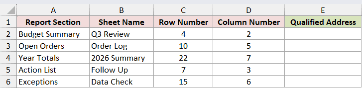
I want to create a fully qualified address for every report section.
Here is the formula:
=ADDRESS(C2:C6,D2:D6,1,TRUE,B2:B6)
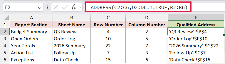
The formula returns addresses such as 'Q3 Review'!$B$4 and 'Order Log'!$E$10. Excel adds single quotation marks around sheet names that contain spaces.
Because each argument covers five rows, one formula spills five qualified addresses into E2:E6.
Example 5: Build Range References from Two Addresses
You can join two ADDRESS results with a colon to create range text.
Below is a list of print sections with start and end coordinates.
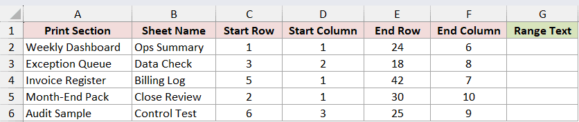
I want to create the full range text for each print section.
Here is the formula:
=ADDRESS(C2:C6,D2:D6,1,TRUE,B2:B6)&":"&ADDRESS(E2:E6,F2:F6,1,TRUE)
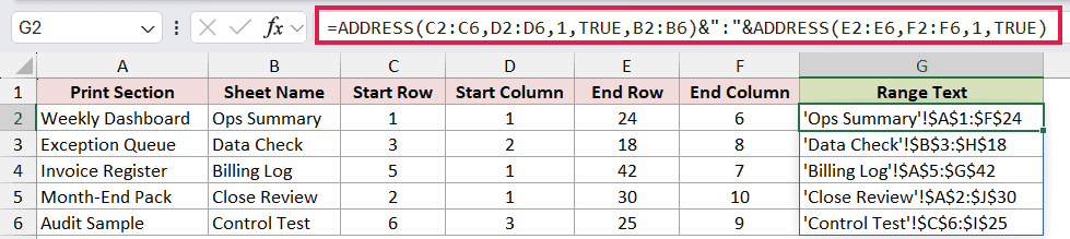
The first ADDRESS result includes the sheet name. The second supplies the ending cell, and the colon joins them into valid range text.
For example, the Weekly Dashboard row returns 'Ops Summary'!$A$1:$F$24. The remaining rows spill beneath it, ending with 'Control Test'!$C$6:$I$25.
This output is still text. If you need an actual reference inside a calculation, INDEX can often create it without converting text.
Example 6: Retrieve a Value from a Generated Address
ADDRESS returns text, but INDIRECT can turn that text into a reference.
Below is an inventory list. The target coordinates are row 5 and column 2.
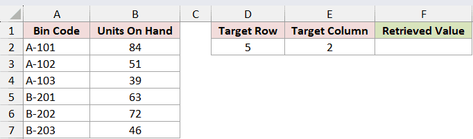
I want to retrieve the value stored at that location.
Here is the formula:
=INDIRECT(ADDRESS(D2,E2,4))
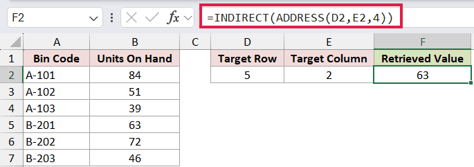
ADDRESS creates the text B5. The INDIRECT function converts it into a live reference, so the formula returns 63 from cell B5.
INDIRECT is volatile, which means Excel recalculates it whenever the workbook recalculates. When the row and column numbers are known, the INDEX function is usually a cleaner option. In this example, =INDEX(A:B,D2,E2) also returns 63.
Tips & Common Mistakes
- ADDRESS returns reference text. It does not retrieve the cell’s value unless another function, such as INDIRECT, converts the text into a reference.
- If you omit
abs_num, Excel returns an absolute reference, such as$F$18. - If you omit
a1, Excel uses A1 notation. Set it to FALSE when you specifically need R1C1 notation. - If you omit
sheet_text, the result does not include a worksheet name. - Sheet names containing spaces appear inside single quotation marks. ADDRESS adds those marks automatically.
- Microsoft lists ADDRESS for Excel 2016 and later.
- In Excel 365, aligned ranges spill cleanly. A blocked output area returns
#SPILL!, while implicit intersection reduces a range formula to one result. - In older Excel versions without dynamic arrays, enter one ADDRESS formula per row and copy it down.
I’ve shown you how to create cell and range addresses, switch reference styles, add sheet names, and turn address text into a usable reference. I hope you found this article helpful.
Related Excel Functions / Articles:
