
The CELL function in Excel returns information about a cell, such as its address, contents, or formatting.
It can help formulas inspect their source cells or display workbook details. The requested information type determines the result, and some types are unavailable on certain platforms.
In this article, I’ll show you how to inspect data types and number formats, return a workbook’s location, and check how negative numbers are formatted.
CELL Function Syntax in Excel
Here is the syntax of the CELL function:
=CELL(info_type,[reference])
info_typeis the kind of information you want. Enter it as quoted text, such as"address","contents", or"format".[reference]is the cell you want to inspect. This argument is optional, but I recommend including it so the result does not depend on whichever cell is active during calculation.
Available information types include address, column, color, contents, filename, format, parentheses, prefix, protection, row, type, and width.
Some information types are platform-specific. Microsoft notes that color, filename, format, parentheses, prefix, protect, and width are not supported in Excel for the web, Excel Mobile, or Excel Starter.
When to Use CELL Function
Use CELL when you need to:
- Return the address, row, column, value, or data type of a cell.
- Check whether imported entries are numeric before using them.
- Inspect the code Excel associates with a built-in number format.
- Display the saved workbook path, file name, and worksheet name.
- Compare a formula’s calculated value with the formula text.
- Detect a number format that displays negative values in red.
Example 1: Return Different Types of Cell Information
CELL can return several kinds of information about the same referenced cell.
The ticket list below contains five statuses. The small table on the right will inspect cell B4, which contains the text Resolved.
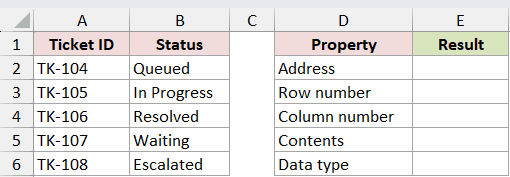
I first want the absolute address of B4 as text.
Here is the formula:
=CELL("address",B4)
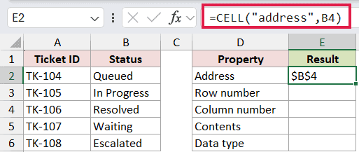
The formula returns $B$4. If you need to construct addresses from row and column numbers, my guide to getting a cell address covers other formula options.
Next, I want the row number.
=CELL("row",B4)
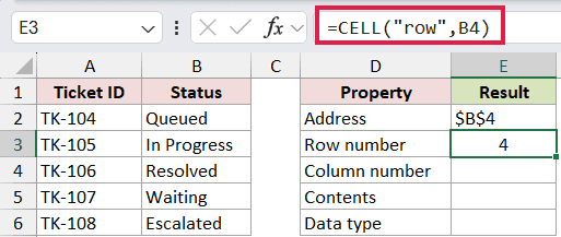
This returns 4 because B4 is in row 4.
I can get its column number in the same way.
=CELL("col",B4)
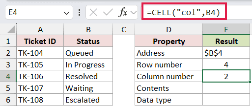
This returns 2 because column B is the second column.
To return the value stored in B4, I use the contents information type.
=CELL("contents",B4)
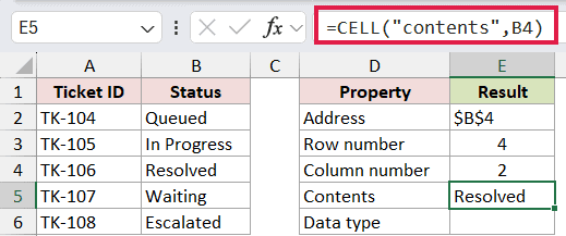
The result is Resolved, the value in B4.
Finally, I want to identify the value’s data type.
=CELL("type",B4)
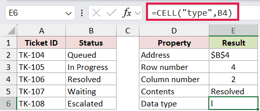
CELL returns l, which means label or text. The other type codes are b for a blank cell and v for anything else, including numbers and formula results.
Example 2: Flag Imported Values That Are Not Numeric
Imported columns often mix proper numbers with notes or blanks.
This import log contains valid amounts, text such as 980 pending, and one empty cell.
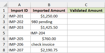
I want to keep numeric amounts and label every other entry for review.
Here is the formula in C2:
=IF(CELL("type",B2)="v",B2,"Review")
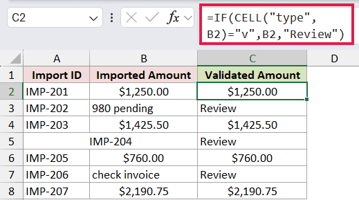
Fill the formula down through C8. When CELL returns v, IF passes the original amount through. Text and blank cells return Review.
The first, third, fifth, and seventh imports remain numeric. The other three rows are flagged. For a clearer array-friendly test, the ISNUMBER function is usually the better choice in a new workbook.
Pro Tip: CELL’s type code v also includes logical values, errors, and formula results. Use ISNUMBER when you specifically need to confirm that a value is numeric.
Example 3: Inspect Number Format Codes
CELL can report a compact code for a cell’s built-in number format.
The dataset below uses General, zero-decimal, two-decimal, and percentage formats in B2:B5.
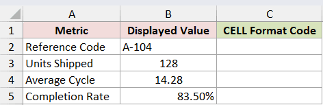
I want to return the format code beside each displayed value.
Here is the formula in C2:
=CELL("format",B2)
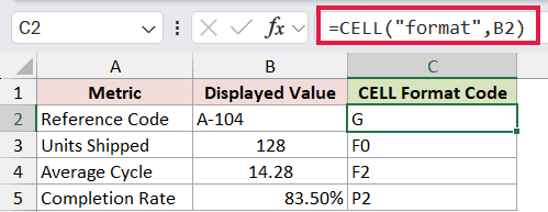
Fill the formula down through C5. The results are G for General, F0 for zero decimals, F2 for two decimals, and P2 for a percentage with two decimals.
These are CELL codes, not the complete custom format strings shown in the Format Cells dialog box. If you change a referenced cell’s format, press F9 to recalculate and update the CELL result.
Example 4: Return the Saved Workbook and Sheet Location
The filename information type returns a workbook’s full saved location together with its worksheet name.
The small setup below has a label in A1 and an empty result cell beside it.

I want to display the location of the workbook that contains A1.
Here is the formula:
=CELL("filename",A1)
The result contains the full folder path, followed by the workbook name in brackets and the current worksheet name after it.
An unsaved workbook returns empty text instead. Save the file, then recalculate if the result stays blank. When you only need a sheet list, there are simpler ways to get sheet names in Excel.
Example 5: Compare a Cell’s Value with Its Formula Text
CELL with the contents information type returns a formula’s result, not the formula itself.
This time sheet contains regular hours, overtime hours, and three result rows that let us compare the two outputs.
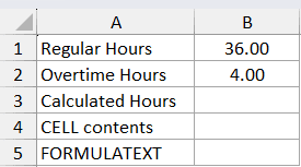
I first calculate the total hours in B3.
=SUM(B1:B2)
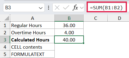
The formula adds 36 regular hours and 4 overtime hours, returning 40.
Next, I ask CELL for the contents of B3.
=CELL("contents",B3)
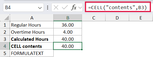
CELL also returns 40 because contents means the calculated value of the referenced cell.
To return the actual formula as text, I use FORMULATEXT.
=FORMULATEXT(B3)
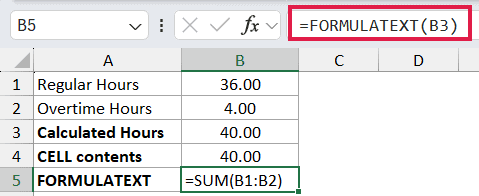
FORMULATEXT returns =SUM(B1:B2) as a text string. It matches what Excel displays in the Formula Bar when B3 is selected.
Example 6: Detect a Red Negative Number Format
CELL can identify number formats that display negative values in a color.
The variance report below alternates between red-negative currency formats and ordinary negative currency formats.
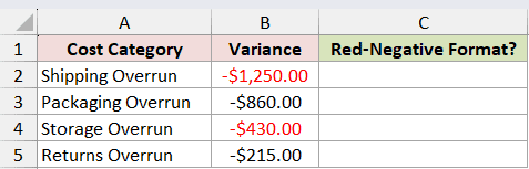
I want to return 1 for the red-negative formats and 0 for the others.
Here is the formula in C2:
=CELL("color",B2)
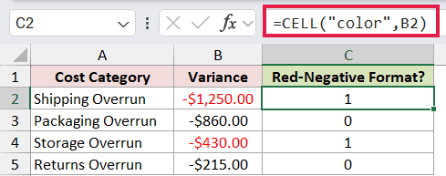
Fill the formula down through C5. The results are 1, 0, 1, and 0, matching the number formats applied to the four variance cells.
The result reads the negative-number format rule. It does not test the current value’s sign or detect font color applied manually or by conditional formatting.
If the goal is simply to control how negative values look, you can also show negative numbers in parentheses or apply another number format directly.
Tips & Common Mistakes
- Put
info_typein double quotation marks. An unquoted word such asaddresscauses a #NAME? error unless that name exists in the workbook. - Include the reference argument. If you omit it, recalculation can return information about whichever cell is active, and that behavior varies by Excel platform.
- CELL does not reliably spill one result per item from a range. Use a single-cell reference and fill the formula down.
- The filename result is blank until the workbook has been saved.
- The format and color information types describe cell formatting, not the displayed text or a conditional-formatting result.
- Press F9 after changing a referenced cell’s format because the CELL result may not update immediately.
- CELL information-type words are language-specific. A formula created in one language version of Excel may return an error in another language version.
- Several format-related information types are unavailable in Excel for the web and mobile versions.
I covered location details, imported-value checks, format codes, saved workbook paths, formula inspection, and red-negative formats. I hope you found this article helpful.
Related Excel Functions / Articles:
