
Excel’s CEILING.MATH function returns a number rounded up to the nearest integer or a specified multiple. Its optional mode argument controls the rounding direction for negative numbers.
It works well for quantities that must cover a requirement, such as tables, storage blocks, billing intervals, or work crews.
In this article, I’ll show you how to round time to quarter hours, calculate whole crews needed, and control rounding for negative numbers with CEILING.MATH.
CEILING.MATH Function Syntax in Excel
The CEILING.MATH function has one required argument and two optional arguments.
=CEILING.MATH(number, [significance], [mode])
numberis the value you want to round.significanceis the multiple to which Excel rounds. It is optional and defaults to 1.modecontrols negative-number rounding. If omitted or zero, Excel rounds toward zero. Any nonzero value rounds away from zero.
When to Use CEILING.MATH Function
- Round a positive decimal up to the next whole number.
- Reserve enough capacity in fixed-size blocks.
- Move a duration up to the next billing interval.
- Convert a workload calculation into a whole resource count.
- Choose whether negative values round toward or away from zero.
Example 1: Round Table Estimates Up
Let’s start with the default integer rounding.
Below is the dataset with events, fractional table estimates, and the whole number of tables to set.
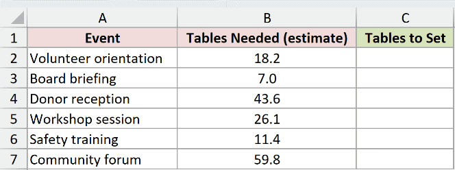
We want to round every table estimate up so each event has enough tables.
Here is the formula:
=CEILING.MATH(B2:B7)
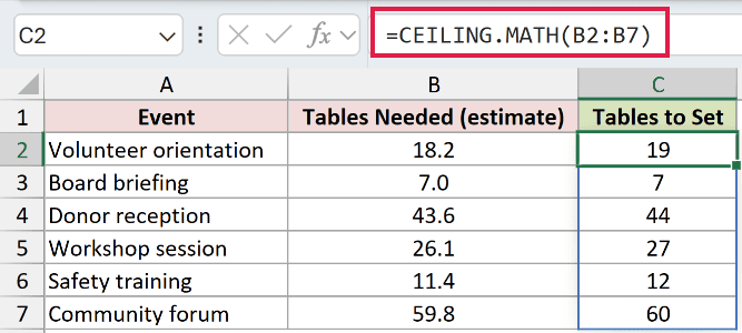
Because significance is omitted, Excel uses 1. The estimates 18.2, 43.6, and 59.8 become 19, 44, and 60.
An estimate that is already a whole number stays unchanged, so 7 remains 7.
In Excel 2021, Excel 2024, and Microsoft 365, the range formula spills all six answers from C2. In Excel 2019 and earlier, use a per-row formula.
Pro Tip: Keep the cells below C2 empty. Any value blocking the spill range causes a #SPILL! error.
Example 2: Reserve Storage in Blocks
Storage reservations often come in fixed blocks.
Below is the dataset with archive sizes, reserved storage, and a 25 GB allocation block in cell F2.
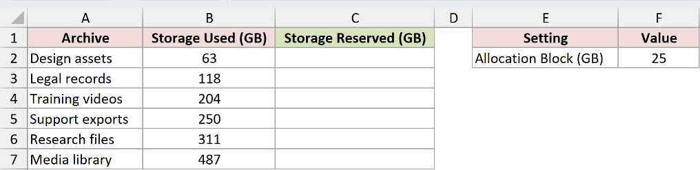
We want to reserve enough storage for each archive using complete 25 GB blocks.
Here is the formula:
=CEILING.MATH(B2:B7,$F$2)
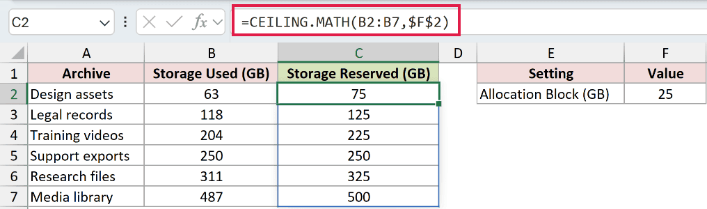
The absolute reference $F$2 supplies 25 as the multiple.
Excel rounds 63 GB to 75 GB, 118 GB to 125 GB, and 204 GB to 225 GB.
An archive already on a 25 GB boundary does not change. The 250 GB support export therefore remains 250 GB.
Pro Tip: The significance argument is a multiple, not a number of decimal places. A significance of 25 returns multiples such as 75, 125, and 225.
Example 3: Round Time to Quarter Hours
The same function can round Excel time values.
Below is the dataset with service tickets, logged durations, and billable durations.
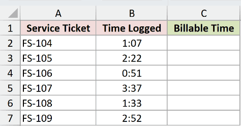
We want to move each logged duration up to the next 15-minute billing interval.
Here is the formula:
=CEILING.MATH(B2:B7,TIME(0,15,0))
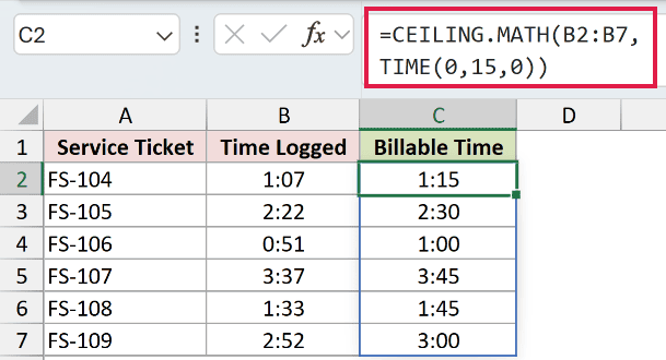
Excel stores time as a fraction of a day. TIME(0,15,0) returns the fraction for 15 minutes and uses it as the rounding multiple.
The logged times 1:07, 2:22, and 3:37 become 1:15, 2:30, and 3:45. This moves each value upward rather than to the nearest quarter hour.
Pro Tip: Format both the source and result cells as time. Changing the number format alters the display, not the stored duration.
Example 4: Calculate Whole Crews Required
CEILING.MATH can also wrap a calculation.
Below is the dataset with project workloads, the hours each crew can handle, and the crews required.
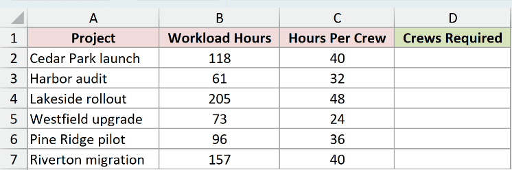
We want to divide each workload by crew capacity and round the result up to a whole crew.
Here is the formula:
=CEILING.MATH(B2:B7/C2:C7)
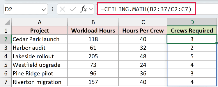
For Cedar Park, 118 divided by 40 is 2.95, so Excel returns 3 crews. Lakeside needs 205 divided by 48, which rounds up to 5 crews.
Riverton returns 4 because 157 hours cannot fit into three 40-hour crew allocations.
Pro Tip: Use CEILING.MATH when a partial resource is not practical. Rounding this quotient down would leave some workload uncovered.
Example 5: Control Negative Number Rounding
Negative numbers are where the mode argument matters.
Below is the dataset with return adjustments and results for the default direction and mode 1.
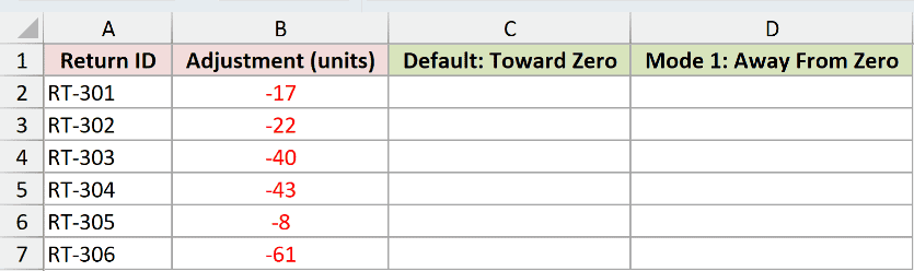
We want to compare rounding negative adjustments to multiples of 5 with and without a nonzero mode.
Here is the default formula:
=CEILING.MATH(B2:B7,5)
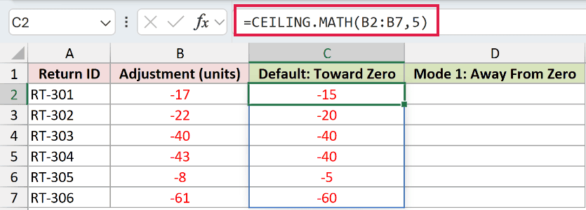
With mode omitted, Excel rounds negative values toward zero. The adjustments -17 and -22 therefore return -15 and -20.
Here is the formula with mode 1:
=CEILING.MATH(B2:B7,5,1)
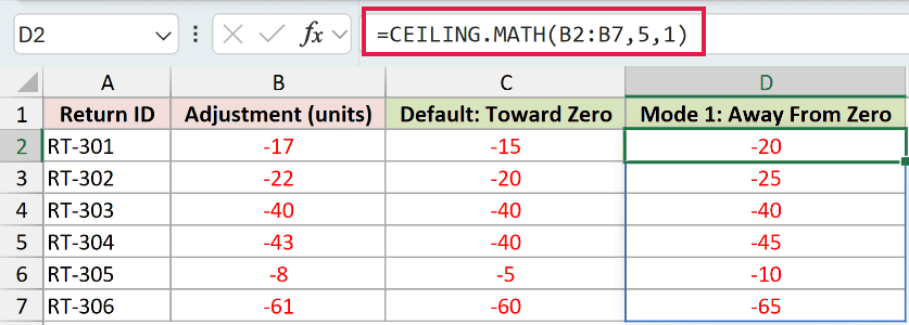
A nonzero mode reverses the direction for negative numbers. The same -17 and -22 adjustments now round away from zero to -20 and -25.
Exact multiples do not change in either column. The -40 adjustment remains -40.
Pro Tip: The mode argument affects only negative numbers. Positive numbers round upward the same way whether mode is zero or nonzero.
Tips & Common Mistakes
- CEILING.MATH rounds to a multiple. Use MROUND when you want the nearest multiple, which can be above or below the original number.
- Use FLOOR.MATH when positive values must round down to an integer or specified multiple.
- ROUNDUP uses a number of digits, while CEILING.MATH uses a multiple. They solve different rounding tasks even when both return a larger positive number.
- CEILING.PRECISE behaves like CEILING.MATH with negative values rounding toward zero, but it has no
modeargument. - The older CEILING function is kept mainly for compatibility. CEILING.MATH was introduced in Excel 2013 and makes negative-number direction explicit.
- An exact multiple stays unchanged. CEILING.MATH does not add another block when the value already meets the boundary.
I covered integer rounding, fixed multiples, time intervals, resource counts, and both directions available for negative numbers.
I hope you found this article helpful.
Related Excel Functions / Articles:
