
Excel’s CEILING function rounds a number to a specified multiple. For positive numbers and a positive multiple, it rounds upward.
It is useful for allowing enough packs, units, or time blocks to cover a requirement. Negative-number behavior depends on the signs of the arguments.
In this article, I’ll show you how to round orders to full cases, round time upward to quarter-hours, and control rounding for negative numbers.
CEILING Function Syntax in Excel
Here is the syntax of the CEILING function:
=CEILING(number, significance)
numberis the value you want to round. This argument is required.significanceis the multiple to which you want to round. This argument is required.
For positive numbers, CEILING rounds up to the next multiple of significance. If the number is already an exact multiple, it remains unchanged.
Negative numbers need extra care. A positive significance rounds a negative number toward zero, while a negative significance rounds it away from zero. CEILING.MATH is the modern alternative when you want explicit control over that direction.
When to Use CEILING Function
Use CEILING when you need to:
- Buy supplies only in full packs or cases.
- Bill time in fixed increments.
- Raise prices to an allowed currency increment.
- Calculate how many whole containers or vehicles are required.
- Apply a configurable rounding multiple to several values.
- Control how negative values round relative to zero.
Example 1: Round Orders to Full Cases
Buying too few units is not an option when a supplier sells only full cases.
The dataset below lists six supplies, the units needed, and the available case size.
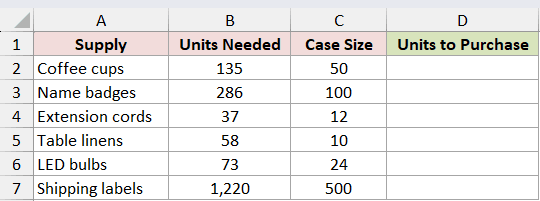
I want to round every required quantity up to a full-case multiple.
Here is the formula:
=CEILING(B2:B7,C2:C7)
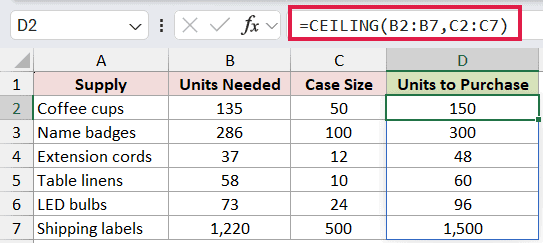
CEILING pairs each quantity in column B with its case size in column C. The results spill into D2:D7.
For example, 135 coffee cups round up to 150 because cases contain 50. The 37 extension cords require 48 units because the next multiple of 12 is 48.
CEILING.MATH produces the same results for these positive values. The original CEILING function remains useful in existing workbooks and formulas.
Pro Tip: CEILING returns a quantity, not a case count. Divide the rounded quantity by the case size if you also need to know how many cases to order.
Example 2: Round Time to 15 Minutes
Time values are numbers in Excel, so CEILING can round them to billing increments.
This service log contains six call durations in column B.
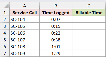
I want to round every duration up to the next 15-minute block.
Here is the formula:
=CEILING(B2:B7,TIME(0,15,0))
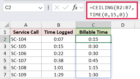
TIME returns the decimal-day value for 15 minutes, which CEILING uses as the significance. The results spill into C2:C7 and use an hours-and-minutes number format.
The 7-minute call rounds to 0:15, the 22-minute call rounds to 0:30, and the 89-minute call rounds to 1:30.
SC-105 displays 0:15 in the source column but returns 0:30. Its stored decimal value is fractionally greater than 15 minutes, even though the cell format hides that difference.
Pro Tip: If a displayed boundary value jumps to the next block, inspect the stored time at higher precision. A tiny hidden fraction can make the value larger than the apparent boundary.
For other rounding directions and methods, see my guide to rounding time to the nearest quarter hour.
Example 3: Round Prices Up to a Nickel
CEILING can also enforce an upward price increment.
The market list below contains calculated prices that must be posted in five-cent increments.
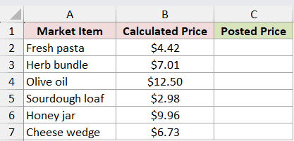
I want to round each price upward to the next multiple of $0.05.
Here is the formula:
=CEILING(B2:B7,0.05)
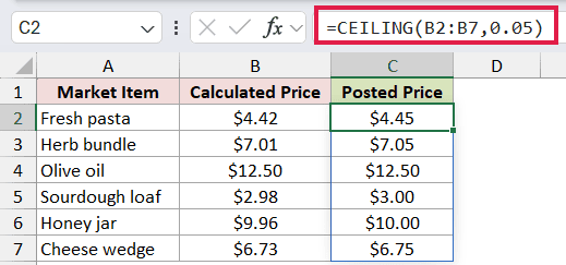
The significance of 0.05 tells CEILING to use nickel-sized steps. Fresh pasta moves from $4.42 to $4.45, while the $12.50 olive oil price remains unchanged because it is already a multiple of $0.05.
Honey moves from $9.96 to $10.00 because $10.00 is the next available five-cent boundary. CEILING never rounds a positive price down.
If you need to choose between upward and downward five-unit rounding, my guide to rounding up or down to the nearest 5 explains the difference.
Example 4: Calculate Whole Vans Needed
Capacity planning often requires a whole number of vehicles.
This moving schedule lists total shipment weight and the weight limit for each assigned van type.
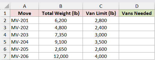
I want to calculate the minimum number of whole vans needed for each move.
Here is the formula:
=CEILING(B2:B7/C2:C7,1)
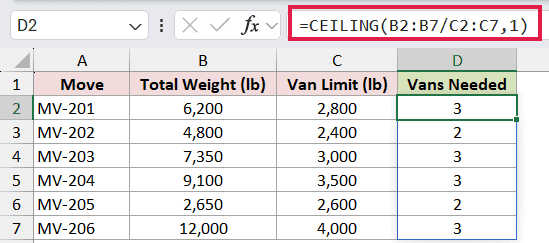
The division calculates a raw vehicle requirement for each row. CEILING then rounds that result up to a multiple of 1, which gives a whole van count.
Move MV-201 needs 6,200 pounds of capacity. Dividing by 2,800 gives about 2.21, so the formula returns 3 vans. MV-202 divides evenly and returns 2.
You can also use =ROUNDUP(B2:B7/C2:C7,0) for this whole-number calculation.
See the ROUNDUP function or my broader guide to rounding up to the nearest whole number for more examples.
Example 5: Use a Cell for Significance
A worksheet setting is easier to maintain than a number repeated inside every formula.
The workspace table below shows storage used in column B. Cell F2 contains the 25 GB billing block.
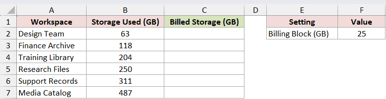
I want to round each storage total up using the billing block stored in F2.
Here is the formula:
=CEILING(B2:B7,$F$2)
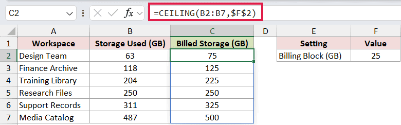
The absolute reference $F$2 keeps the significance fixed at 25 GB for every value in the spilled calculation.
Design Team’s 63 GB rounds to 75 GB, Finance Archive’s 118 GB rounds to 125 GB, and the 250 GB Research Files value remains 250 because it already matches a billing boundary.
Change F2 and the entire result column recalculates with the new block size. CEILING.MATH can use the same cell reference if you later replace the legacy function.
Example 6: Control Negative Rounding Direction
The sign of the significance changes how legacy CEILING handles negative numbers.
This warehouse report contains negative stock variances in column B. Columns C and D show the two possible directions in multiples of 5.
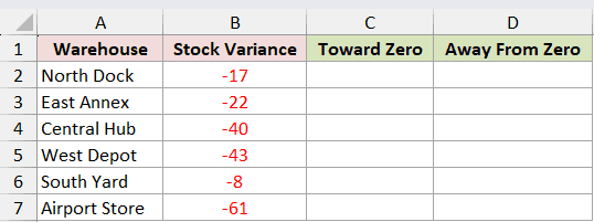
I first want to round each variance toward zero.
Here is the formula:
=CEILING(B2:B7,5)
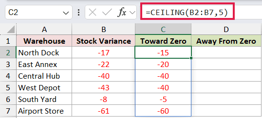
With a positive significance, -17 rounds toward zero to -15. A value already divisible by 5, such as -40, stays unchanged.
Next, I want to round the same variances away from zero.
Here is the formula:
=CEILING(B2:B7,-5)
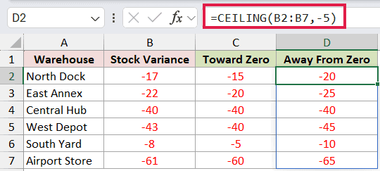
With a negative significance, -17 rounds away from zero to -20. Across the two spilled columns, -61 becomes -60 toward zero and -65 away from zero.
For a modern formula with a dedicated direction argument, =CEILING.MATH(B2:B7,5) rounds toward zero by default. Use =CEILING.MATH(B2:B7,5,1) to round negative values away from zero.
Tips & Common Mistakes
- CEILING rounds positive numbers upward to a multiple. The ROUND function instead chooses the nearest value and can round down.
- MROUND is not a substitute when you must always round upward. It returns the nearest multiple, which may be below the original number.
- Exact multiples do not change. This applies to quantities, prices, time values, and negative numbers.
- Nonnumeric arguments return #VALUE!.
- In current dynamic array versions of Excel, range arguments spill. Keep the result area empty to avoid a #SPILL! error.
- For new formulas, consider CEILING.MATH. Its optional mode argument makes negative-number direction easier to control and understand.
I covered full cases, quarter-hour billing, nickel prices, whole vehicles, cell-based significance, and negative rounding. I hope you found this article helpful.
Related Excel Functions / Articles:
