
MAPE (mean absolute percentage error) in Excel shows you how far your forecasts missed actual results, as an average percentage. Over- and under-forecasts don’t cancel each other out.
Months with zero actual sales break the usual MAPE formula.
I’ll show you how to calculate MAPE with a helper column, a single formula, and SUMPRODUCT, then handle zero months and calculate WAPE.
What Is MAPE?
When you compare actual sales with your forecast, you can express each month’s miss as a percentage of actual sales. MAPE averages those percentages.
MAPE stands for mean absolute percentage error. In words, the formula is the average of absolute error divided by actual value, shown as a percentage.
A MAPE of 4.5% means your forecasts were off by about 4.5% of actual sales on average. Lower is better.
Method #1: Using a Helper Column With ABS and AVERAGE
A helper column lets you see each month’s percentage error before you calculate the average. I’d use this when you want to spot the biggest misses.
Below I have a dataset showing an online store’s Month, Actual Sales, and Forecast Sales for January through December 2025.
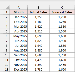
Use B2:B13 for actual sales and C2:C13 for forecasts. You want one MAPE value for all 12 months.
Type Absolute % Error in D1, then enter this formula in D2:
=ABS((B2:B13-C2:C13)/B2:B13)
Select D2:D13, then choose Home tab > Percent Style or press Ctrl+Shift+%. Click Increase Decimal once to show one decimal place.
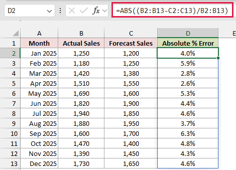
In Microsoft 365 and Excel 2021 or later, the formula spills down to D13 automatically. Keep D3:D13 empty so there’s room for the results.
B2:B13-C2:C13 calculates actual sales minus forecast sales for each month. A negative result means you forecast too much.
Dividing by B2:B13 expresses each error as a share of actual sales. ABS removes the minus signs so overestimates and underestimates don’t cancel out.
For January, you sold 1,250 units and forecast 1,200. The 50-unit miss is 4.0% of actual sales.
In Excel 2019 and older, enter =ABS((B2-C2)/B2) in D2 and copy it down to D13.
To calculate MAPE, type MAPE in F1 and enter this formula in F2:
=AVERAGE(D2:D13)
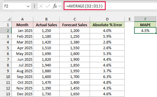
AVERAGE calculates the mean of the 12 absolute percentage errors. Format F2 as a percentage with one decimal place, and you’ll see 4.5%.
You can also see September had the biggest miss at 6.3%. April had the smallest at 2.6%.
Method #2: Using a Single AVERAGE and ABS Formula
You can put the whole calculation in one cell. I recommend this method for most Microsoft 365 readers because you don’t need a helper column.
Below I have a dataset showing an online store’s Month, Actual Sales, and Forecast Sales for January through December 2025.
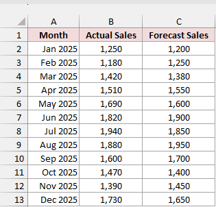
For these 12 months, compare the forecasts in C2:C13 with actual sales in B2:B13 to find the average percentage error.
Type MAPE in E1, then enter this formula in E2. In Microsoft 365 or Excel 2021 or later, press Enter:
=AVERAGE(ABS((B2:B13-C2:C13)/B2:B13))
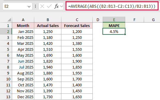
Format E2 as a percentage with one decimal place. Your MAPE is 4.5%.
How does this formula work?
Excel subtracts each forecast from its actual value and divides the difference by that actual value. ABS removes any minus signs from the percentage errors.
AVERAGE then combines those 12 errors into one result. You get the same MAPE as the helper-column method, with the intermediate calculations inside the formula.
Note: In Excel 2019 and older, confirm this formula with Ctrl+Shift+Enter. Pressing Enter alone can return a wrong result or #VALUE!.
Method #3: Using the SUMPRODUCT Function
If you’re using an older Excel version, SUMPRODUCT handles the calculation without Ctrl+Shift+Enter. It also works in newer versions.
Below I have a dataset showing an online store’s Month, Actual Sales, and Forecast Sales for January through December 2025.
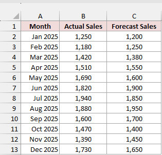
B2:B13 contains actual sales, while C2:C13 contains forecasts. You’ll average the percentage errors for all 12 months.
Type MAPE in E1, then enter this formula in E2 and press Enter:
=SUMPRODUCT(ABS((B2:B13-C2:C13)/B2:B13))/COUNT(B2:B13)
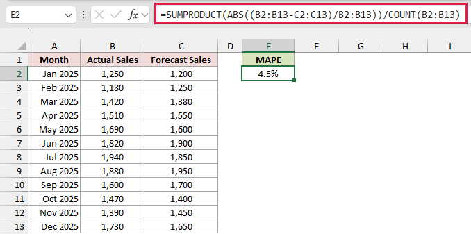
Format E2 as a percentage with one decimal place. This formula also returns 4.5%.
How does this formula work?
SUMPRODUCT usually multiplies arrays and adds the results. With only one array here, it adds up the absolute percentage errors.
COUNT(B2:B13) counts the 12 months with numeric actual sales.
Dividing the total error by 12 gives you the average. SUMPRODUCT handles arrays on its own, so this works in every Excel version without Ctrl+Shift+Enter.
How to Calculate Forecast Accuracy From MAPE
Many teams report forecast accuracy by subtracting MAPE from 100%. You can calculate that alongside your MAPE result.
For the online store’s 12 monthly sales figures, actual sales are in B2:B13 and forecasts are in C2:C13.
Type MAPE in E1. In E2, enter =AVERAGE(ABS((B2:B13-C2:C13)/B2:B13)), the formula from Method #2, which returns 4.5% for this data.
In Excel 2019 and older, confirm this formula with Ctrl+Shift+Enter.
Type Forecast Accuracy in F1, then enter this formula in F2:
=1-E2
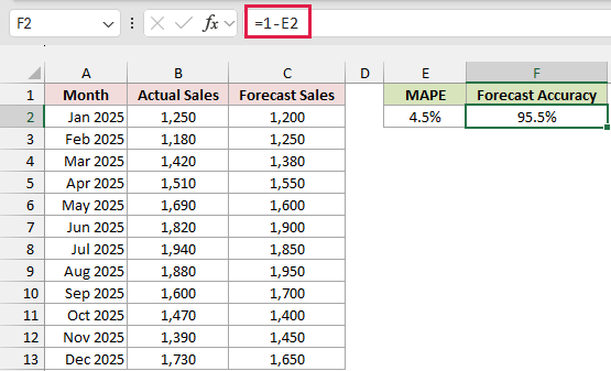
Format both results as percentages with one decimal place. E2 shows 4.5% MAPE, and F2 shows 95.5% forecast accuracy.
If MAPE goes above 100%, this calculation turns negative. To keep your reported accuracy at a minimum of 0%, use this formula in F2:
=MAX(0,1-E2)
How to Calculate MAPE When Actual Values Include Zero
A month with no sales breaks the usual MAPE formula because it divides each error by actual sales. You can skip those months, but there’s a trade-off.
Below I have a dataset of monthly space heater sales, with Month, Actual Sales, and Forecast Sales. Actual sales are zero in June, July, and August.
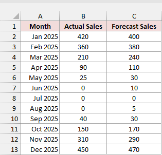
The heater sales in B2:B13 are the actuals; C2:C13 has the forecasts. Calculate MAPE for the months when heaters sold.
Type MAPE in E1. If you enter the Method #2 formula in E2, it returns #DIV/0! because those three actual values are zero:
=AVERAGE(ABS((B2:B13-C2:C13)/B2:B13))
In Excel 2019 and older, confirm this formula with Ctrl+Shift+Enter.
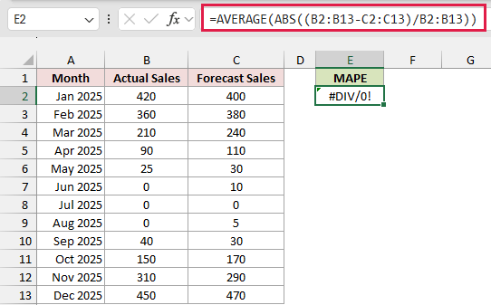
To leave the zero months out, replace the formula in E2 with this one:
=AVERAGE(IF(B2:B13<>0,ABS((B2:B13-C2:C13)/B2:B13)))
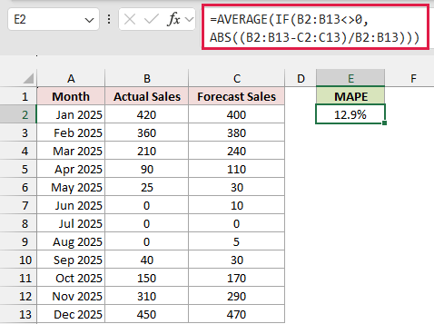
Press Enter in Microsoft 365 or Excel 2021 or later. In Excel 2019 and older, use Ctrl+Shift+Enter. Format E2 as a percentage with one decimal place.
The result is 12.9%, based on the nine months with non-zero actual sales.
How does this formula work?
IF checks whether each actual value is non-zero. For those months, it calculates the absolute percentage error.
For zero months, IF returns FALSE instead of the division result, so no #DIV/0! error reaches AVERAGE.
AVERAGE ignores those FALSE values, so only the nine non-zero months count.
This also leaves out the misses in zero months entirely. June’s forecast of 10 units and August’s forecast of 5 units don’t affect your MAPE.
How to Calculate Weighted MAPE (WAPE) in Excel
I’d use WAPE when you want busy months to count more than quiet ones, or you want forecast misses in zero-sales months included.
Below I have a dataset of monthly space heater sales, with Month, Actual Sales, and Forecast Sales, including three summer months with zero actual sales.
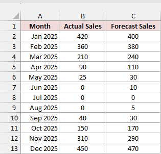
With actual sales in B2:B13 and forecasts in C2:C13, you’ll measure total absolute forecast error as a percentage of total sales.
Type WAPE in E1, then enter this formula in E2:
=SUMPRODUCT(ABS(B2:B13-C2:C13))/SUM(B2:B13)
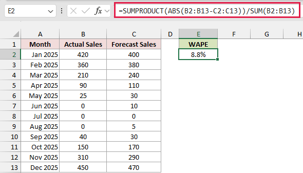
Format E2 as a percentage with one decimal place. Your WAPE is 8.8%. This formula works in every Excel version.
How does this formula work?
SUMPRODUCT adds up all the absolute errors, including misses in zero-sales months. Dividing by SUM(B2:B13) expresses that total error as a share of total actual sales.
You aren’t dividing by each month’s sales, so individual zeros are fine. The total actual sales must still be greater than zero.
This calculation is also called weighted MAPE or WMAPE. Larger sales months carry more weight than smaller ones.
That’s why WAPE is lower than the 12.9% MAPE here. April’s 20-unit miss against 90 units sold is 22.2%.
September’s 10-unit miss against 40 units sold is 25.0%.
Plain MAPE gives these quiet months the same weight as busy months. WAPE measures their misses against the total sales for the year.
Additional Notes About Calculating MAPE in Excel
- Divide by actual values, not forecasts. Changing the denominator changes what your percentage error measures.
- Keep the actual and forecast ranges the same size, with matching months on each row. Remove blanks and text from actuals. Blanks cause #DIV/0! and text causes #VALUE!.
- For non-negative forecasts, an under-forecast’s error tops out at 100%. An over-forecast has no ceiling, so MAPE penalizes the two directions differently.
- Check the helper column when MAPE looks unusually high. A tiny actual value can produce a huge percentage error and dominate the average.
- Compare MAPE across the same data series and periods. Changing the product mix or including different months can make the scores misleading.
Frequently Asked Questions
Here are a few other questions you might have when measuring forecast error in Excel.
Is There a MAPE Function in Excel?
No, Excel doesn’t have a built-in MAPE function. You need to combine functions to calculate it for your actual and forecast values.
FORECAST.ETS.STAT with statistic_type 5 returns symmetric MAPE, or SMAPE. It only measures Excel’s own exponential smoothing forecast, not forecasts you already have.
What Is a Good MAPE Value?
A rough scale from Colin Lewis’s 1982 forecasting book calls MAPE below 10% highly accurate, 10% to 20% good, 20% to 50% reasonable, and above 50% inaccurate.
Treat those as broad guidelines. What counts as good depends on your industry and how predictable your sales or other values are.
What Is the Difference Between MAPE and MAE?
MAE measures the average absolute error in the original units. For the online store’s actual sales in B2:B13 and forecasts in C2:C13, use:
=AVERAGE(ABS(B2:B13-C2:C13))
In Excel 2019 and older, confirm this formula with Ctrl+Shift+Enter.
This returns 70 units. MAPE expresses each error as a percentage of actual sales, so you can compare forecasts for products that sell very different amounts.
Conclusion
I recommend the single AVERAGE and ABS formula for Microsoft 365 and Excel 2021 or later, and SUMPRODUCT for older versions.
Use a helper column to inspect individual months, and skip zero-sales months or use WAPE to include their misses.
I hope you found this article helpful.
Other Excel articles you may also like:
