
The FVSCHEDULE function in Excel returns the future value of a lump sum after applying a series of changing interest rates.
It compounds each period using that period’s rate, so it suits financial values that do not grow at one constant rate.
In this article, I’ll show you how to use rate schedules, calculate values for several principals, and avoid the average-rate trap.
FVSCHEDULE Function Syntax in Excel
The FVSCHEDULE function takes a starting value and a schedule of rates.
=FVSCHEDULE(principal, schedule)
- principal (required) is the present value or starting amount.
- schedule (required) is the range or array containing the rates to apply, one after another.
When to Use FVSCHEDULE Function
- Calculate the maturity value of a deposit with rates that change each year.
- Apply one escalation schedule to several contract prices.
- Build a year-by-year value history from an expanding rate range.
- Measure cumulative change across a series of inflation or return rates.
- Compound monthly balances when the quoted annual rate changes during the year.
Example 1: Calculate a Step-Up CD Value
Let’s start with a deposit whose rate rises over five years.
Below is the dataset. Column B contains the annual rates, B8 holds the opening deposit, and the labeled cell in B9 will hold the maturity value.
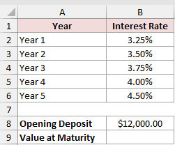
We want to calculate the value of the $12,000 deposit after all five rates have been applied.
Here is the formula:
=FVSCHEDULE(B8,B2:B6)
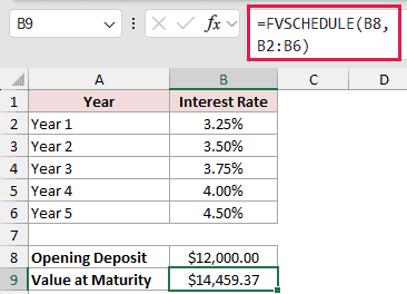
The formula starts with the deposit in B8 and compounds it using the rates in B2:B6. The value at maturity is $14,459.37.
You could reproduce the same result with PRODUCT by multiplying the deposit by each growth factor. FVSCHEDULE replaces those separate multiplications with one function call.
Example 2: Apply One Schedule to Several Prices
The same schedule can update several service contracts.
Below is the dataset. Columns A and B list services and starting prices, column C will hold Year 4 prices, and F2:F4 contains the shared schedule.
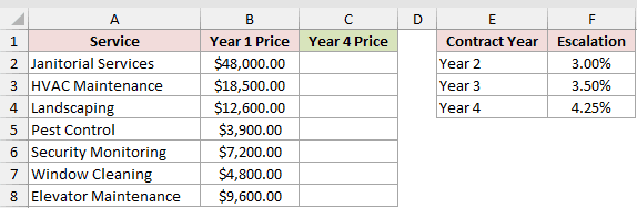
We want to calculate each Year 4 price while keeping the schedule fixed.
Here is the formula entered in C2 and copied down:
=FVSCHEDULE(B2,$F$2:$F$4)
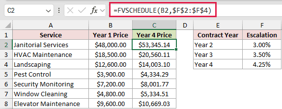
The relative reference B2 changes on each row. The absolute reference $F$2:$F$4 keeps the three escalation rates locked while the formula is copied down.
Janitorial Services rises from $48,000.00 to $53,345.14. Elevator Maintenance rises from $9,600.00 to $10,669.03 under the same schedule.
Pro Tip: Passing a principal range to FVSCHEDULE returns one #VALUE!. In Microsoft 365 or Excel 2024, MAP with LAMBDA can return one result per principal: =MAP(B2:B8,LAMBDA(p,FVSCHEDULE(p,$F$2:$F$4))). MAP returns #NAME? in Excel 2021.
Example 3: Build Year-by-Year Property Values
Here’s a useful way to see the value after every year.
Below is the dataset. Columns A and B contain years and appreciation rates, B9 holds the purchase price, and column C will show each year-end value.
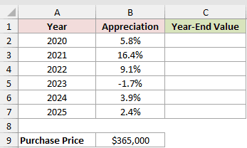
We want each row to include every appreciation rate from 2020 through that row’s year.
Here is the formula entered in C2 and copied down:
=FVSCHEDULE($B$9,$B$2:B2)
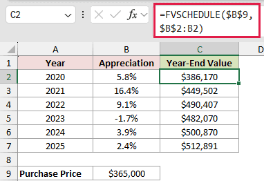
The purchase price stays locked at $B$9. The ending point of $B$2:B2 expands as the formula moves down, adding one rate on each row.
Negative rates work too. The negative 1.7% rate in 2023 reduces the year-end value from $490,407 to $482,070 before growth resumes.
Example 4: Calculate Cumulative Inflation
The same approach can measure cumulative inflation.
Below is the dataset. Column B contains sample inflation rates, B9 holds the earlier salary, and B10:B11 will hold the cumulative rate and adjusted salary.
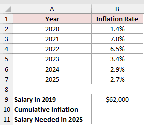
We first want to calculate the cumulative inflation across all six years.
Here is the formula:
=FVSCHEDULE(1,B2:B7)-1
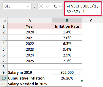
Using 1 as the principal returns the cumulative growth factor. Subtracting 1 converts that factor into a cumulative inflation rate of 26.26%.
We can apply the same rate schedule to the $62,000 salary in B9.
Here is the formula:
=FVSCHEDULE(B9,B2:B7)
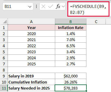
The result is $78,283. That is the salary needed in 2025 to match the cumulative change in this sample schedule.
Pro Tip: These inflation rates are sample data, not official CPI figures. Replace them with the rates that belong to your own analysis.
Example 5: Compound Changing Monthly Rates
Now let’s work with a savings rate that changes during the year.
Below is the dataset. Column B contains each month’s quoted annual rate, B15 holds the opening balance, and B16 will hold the balance after 12 months.
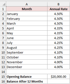
We want to apply each annual quote as a monthly rate before compounding the balance.
Here is the formula:
=FVSCHEDULE(B15,B2:B13/12)
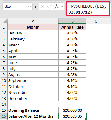
B2:B13/12 converts each annual quote to its monthly rate inside the formula. FVSCHEDULE applies those monthly rates and returns one value, $20,869.35.
The division must match the compounding period. Convert annual quotes to the corresponding per-period rates before passing them to FVSCHEDULE.
Pro Tip: This formula works as written in Excel 2021, Excel 2024, and Microsoft 365. In Excel 2019 and earlier, confirm it with Ctrl+Shift+Enter or use a helper column of monthly rates.
Example 6: Avoid the Average-Return Trap
A variable-return example shows why the average can mislead.
Below is the dataset. Column B contains five sample fund returns, B8 holds the investment, and B9:B10 will hold the actual and average-rate ending values.
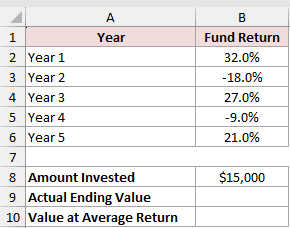
We first want the ending value after applying every annual return.
Here is the formula:
=FVSCHEDULE(B8,B2:B6)
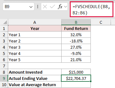
FVSCHEDULE applies each positive and negative return to the $15,000 investment. The actual ending value is $22,704.37.
Here is the FV formula that demonstrates the average-rate mistake:
=FV(AVERAGE(B2:B6),COUNT(B2:B6),0,-B8)
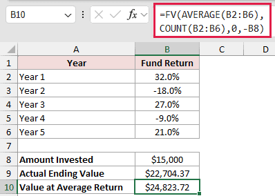
The white cell in B10 shows the mistaken average-rate comparison. Replacing the yearly returns with their average produces $24,823.72.
The comparison overstates the ending value. FVSCHEDULE keeps every observed return in the calculation instead of replacing the schedule with one rate.
Tips & Common Mistakes
- Enter rates as percentages or decimals. Excel reads 2.1 without a percent sign as 210%, so rates of 2.1, 1.5, and 0.8 turn $10,000 into $139,500.
- A blank cell in the schedule counts as 0%. Text in the schedule returns #VALUE!, so select only the rate cells.
- FVSCHEDULE accepts one principal per call. For several principals, copy the formula down with an absolute schedule reference.
- FVSCHEDULE handles one lump sum and has no payment argument. When regular payments are included, use FV only if one constant rate applies.
- The schedule can run vertically or horizontally.
- To annualize Example 6’s returns,
=FVSCHEDULE(1,B2:B6)^(1/COUNT(B2:B6))-1returns 8.64%. This gives you one comparable rate for the RRI function.
Each schedule entry should match one compounding period. Once the rates are in the right order, FVSCHEDULE handles the compounding.
Related Excel Functions / Articles:
