MID Function in Excel

If you want to pull a chunk of text out of the middle of a cell, starting at a specific position and grabbing a set number of characters, the MID function is what you reach for.

In Excel 365, you can also feed MID a range and the results spill into the cells below, so one formula handles the whole column.

In this article I’ll walk through practical MID examples, starting with simple fixed-length codes and working up to pulling values out from between two characters.

MID Function Syntax in Excel

The MID function returns a specific number of characters from a text string, starting at the position you tell it.

=MID(text, start_num, num_chars)

• text – the text string you want to extract characters from.
• start_num – the position of the first character you want to grab (1 is the first character).
• num_chars – how many characters to pull, starting from start_num.

When to Use MID Function

Here are some everyday situations where MID comes in handy:

• Pulling a fixed-length code out of a product ID or SKU.
• Grabbing a segment from the middle of a structured string.
• Extracting text that sits between two markers, like brackets or an @ sign.
• Reading an area code out of a formatted phone number.
• Splitting a tag into its parts when each part starts at a known spot.

Example 1: Extract a Fixed-Length Code from Each SKU

Let’s start with a simple one.

Below is the dataset. Column A has product SKUs that all follow the same pattern, a three-letter category code, then a number, then a single letter.

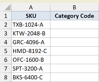
I want to pull just the first three letters from each SKU into column B.

Here is the formula:

=MID(A2:A8,1,3)

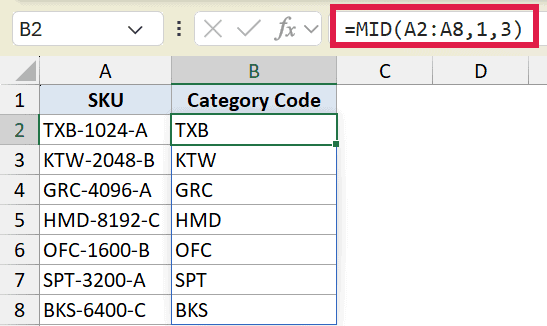
MID starts at position 1 and grabs 3 characters from each SKU. Since I fed it the whole range A2:A8, the results spill down the column from one formula.

Pro Tip: When the part you want sits right at the start, LEFT is the more natural choice. MID works fine too, but =LEFT(A2:A8,3) reads cleaner for anyone reviewing your sheet.

Example 2: Pull a Middle Segment by Position

Here’s another practical scenario.

Below is the dataset. The same product codes are in column A, and this time I want the four-digit batch number that sits in the middle.

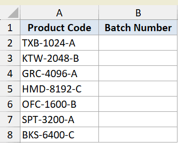
The batch number always starts at the fifth character and runs for four digits, so the positions are fixed.

Here is the formula:

=MID(A2:A8,5,4)

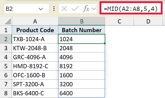
Position 5 skips past the three letters and the first dash, then MID takes the next four characters.

This works because every code has the exact same layout.

Pro Tip: MID by position only works when the part you want is always in the same spot. If the length before it varies, you’ll need FIND or SEARCH to locate the start instead, as in the next examples.

Example 3: Extract Text Between Two Characters

Let’s step it up with something a bit more involved.

Below is the dataset. Column A has order notes where the item name is wrapped in square brackets, and the surrounding text varies in length.

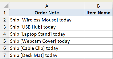
I want to pull out just the item name that sits between the opening and closing brackets.

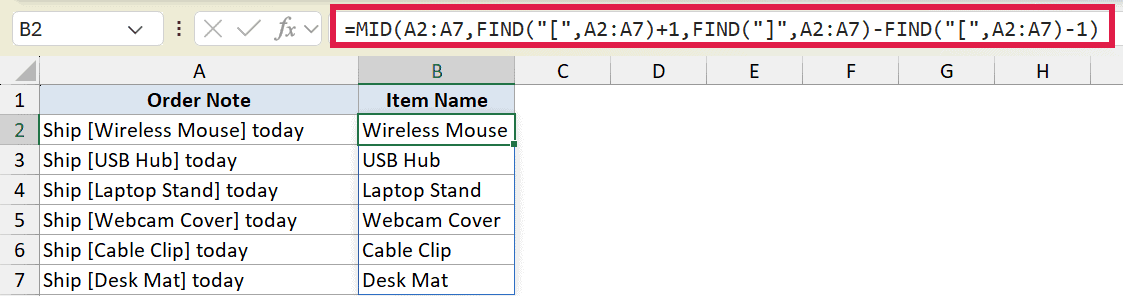
Here is the formula:

=MID(A2:A7,FIND("[",A2:A7)+1,FIND("]",A2:A7)-FIND("[",A2:A7)-1)

How this formula works:

• The FIND function with +1 finds the opening bracket and starts MID on the first character of the name.
• FIND("]",A2:A7)-FIND("[",A2:A7)-1 is the distance between the two brackets, which is how many characters to grab.
• MID then returns everything between the brackets, no matter where they fall.

In Excel 365 you can also do this with TEXTBEFORE and TEXTAFTER: =TEXTBEFORE(TEXTAFTER(A2:A7,"["),"]"). That reads more plainly. The MID version still works in older Excel where those functions don’t exist, so it’s worth knowing both.

Example 4: Extract Text After a Specific Character

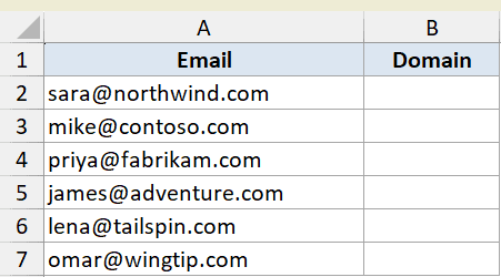
Here’s a common one for anyone working with email lists.

Below is the dataset. Column A has email addresses, and I want the domain, which is everything after the @ sign.

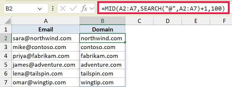
The @ sits at a different position in each address, so I use the SEARCH function to find it first, then grab everything after it.

Here is the formula:

=MID(A2:A7,SEARCH("@",A2:A7)+1,100)

How this formula works:

• SEARCH("@",A2:A7)+1 locates the @ and starts MID on the character right after it.
• The 100 is just a number bigger than any domain will ever be, so MID grabs the rest of the string.
• MID returns whatever’s left, which is the full domain.

In Excel 365 the cleaner option is =TEXTAFTER(A2:A7,"@"). It does the same job without the made-up large number. The MID approach is still handy in older versions and when you want to control exactly how many characters to take.

Example 5: Extract a Number and Convert It

Let’s look at a case where MID alone isn’t quite enough.

Below is the dataset. Column A has invoice tags where the dollar amount sits between two dashes, and I want it as a real number I can total up.

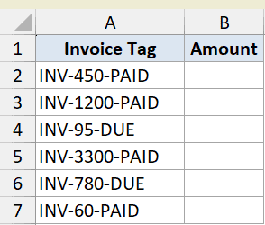
I want to pull the amount out of each tag and have Excel treat it as a number, not text.

Here is the formula:

=VALUE(MID(A2:A7,5,FIND("-",A2:A7,5)-5))

How this formula works:

• The amount always starts at position 5, right after INV-.
• FIND("-",A2:A7,5)-5 measures the gap from there to the next dash, which is the length of the number.
• MID pulls out the digits as text, then VALUE converts that text into an actual number.

Pro Tip: MID always returns text, even when the characters are all digits. If you plan to do math on the result, wrap it in VALUE so Excel treats it as a number rather than a text string.

Example 6: Get the Area Code from Phone Numbers

Let’s finish with phone numbers.

Below is the dataset. Column A has numbers formatted with the area code in parentheses, and I want just those three digits.

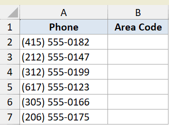
The area code always starts at the second character, right after the opening parenthesis, and runs for three digits.

Here is the formula:

=MID(A2:A7,2,3)

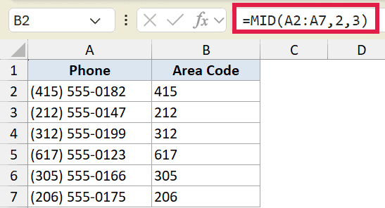
MID starts at position 2 to skip the opening parenthesis, then takes the next three characters. Because every number uses the same format, the fixed positions work for the whole column.

Tips & Common Mistakes

• MID counts from 1, not 0. The first character is position 1. A common slip is starting at 0 and getting an error or a shifted result.
• The result is always text. Even all-digit results come back as text. Wrap MID in VALUE when you need a number for calculations.
• Use FIND or SEARCH for moving targets. When the part you want doesn’t start at a fixed spot, find the position of a character first and feed that position into MID.
• FIND is case-sensitive, SEARCH is not. Pick SEARCH when the marker’s case might vary, FIND when you need an exact match.
• In Excel 365, modern text functions are often simpler. TEXTBEFORE and TEXTAFTER handle delimiter-based extraction more directly. MID is still the go-to in older versions and for position-based grabs.

That covers the main ways to use MID, whether your target sits at a fixed position or needs FIND or SEARCH to locate it first. Most real-world text problems come down to that one question: is the start always in the same place, or does it move?

Once you’re comfortable combining MID with those helper functions, you can extract part of text from almost any structured string in your sheet.

List of All Excel Functions

Related Excel Functions / Articles:

• LEFT Function in Excel
• SEARCH vs FIND Function in Excel
• How to Extract Number from Text in Excel (Beginning, End, or Middle)
• How to Extract First Name in Excel
• Extract ZIP Code from Address in Excel
• Remove Middle Name from Full Name in Excel
• REPLACE Function in Excel
• SUBSTITUTE Function in Excel