
The PDURATION function in Excel returns the number of periods a starting amount needs to reach a target at a constant compound growth rate.
It assumes the amount grows without extra deposits or withdrawals. An annual rate returns years, while a monthly rate returns months, so the rate determines how you read the answer.
In this article, I’ll show you how to calculate savings timelines, handle monthly compounding, and spot negative results that mean a goal is already reached.
PDURATION Function Syntax in Excel
PDURATION uses a growth rate, a starting value, and a target value:
=PDURATION(rate, pv, fv)
- rate (required): The interest or growth rate per compounding period.
- pv (required): The present value, or amount you’re starting with. Enter it as a positive value.
- fv (required): The future value you want to reach. Enter it as a positive value too.
The rate must be positive. PDURATION can return fractional periods, and a target below the starting value produces a negative result.
PDURATION is available in Excel 2013 and later.
When to Use PDURATION Function
- Estimate how long an existing savings balance needs to reach a goal without further deposits.
- Calculate the months needed when an account compounds interest monthly.
- Compare doubling times at different growth rates.
- Project when a subscriber count will reach a target under a constant percentage-growth assumption.
Example 1: Calculate Years to Reach Savings Goals
Let’s start with savings balances that grow through interest alone.
Below is the dataset with savings goals, current balances, target amounts, and annual rates in columns A through D. Column E will hold the years needed.
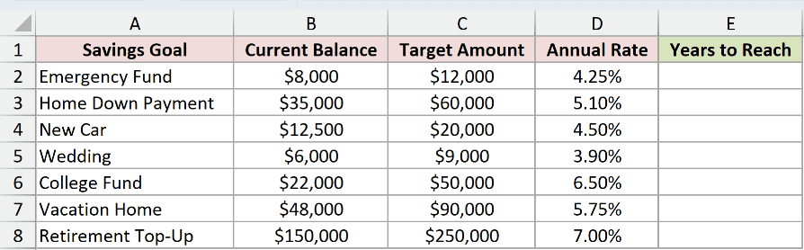
We want to calculate how many years each balance needs to reach its target, assuming annual compounding.
Enter this formula in E2:
=PDURATION(D2:D8,B2:B8,C2:C8)
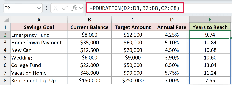
The formula takes each row’s rate from column D, starting balance from column B, and target from column C. Its results spill into E2:E8.
The Emergency Fund grows from $8,000 to $12,000 at 4.25%, returning 9.74 years. The Home Down Payment returns 10.84 years.
The result counts periods. Because these rates apply annually, each period represents a year.
Range formulas spill in Excel 2021, Excel 2024, and Microsoft 365. In Excel 2019 and earlier, use references to each row’s individual cells and copy down.
Pro Tip: Treat the rate as a constant-growth assumption. If the rate changes or you add deposits, the timeline no longer describes the same savings plan.
Example 2: Use PDURATION With Monthly Compounding
The rate needs a conversion when interest compounds monthly.
Below is the dataset with account names, deposits, target balances, and annual rates. Columns E and F will show the time in months and years.
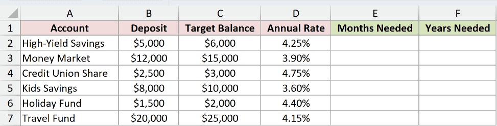
We want the months needed for each deposit to reach its target, using nominal annual rates compounded monthly.
Enter this formula in E2:
=PDURATION(D2:D7/12,B2:B7,C2:C7)
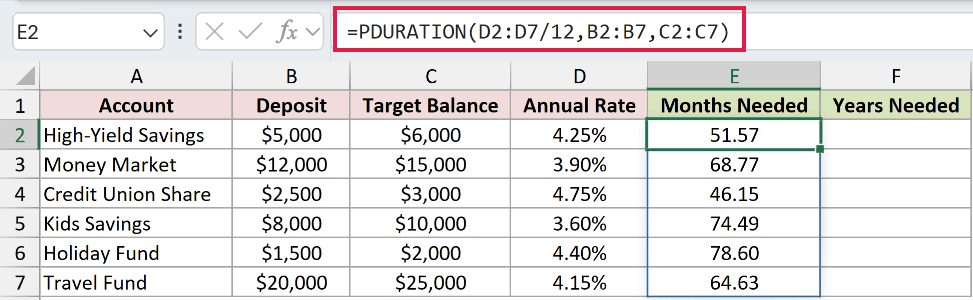
Dividing the annual rates by 12 supplies a monthly rate. PDURATION then returns months, spilling the results into E2:E7.
High-Yield Savings returns 51.57 months for $5,000 to reach $6,000 at the listed 4.25% annual rate. Money Market returns 68.77 months.
To express those same timelines in years, enter this formula in F2:
=E2:E7/12
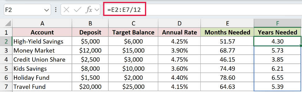
The converted results are 4.30 years for High-Yield Savings and 5.73 years for Money Market. The timeline still uses monthly compounding.
Pro Tip: This setup uses nominal annual rates. Don’t divide an effective annual yield by 12 and treat it as the monthly rate. Confirm how your input rate is stated first.
Example 3: Calculate Doubling Time
You don’t need a particular account balance to calculate doubling time.
Below is the dataset with annual rates in column A. Columns B and C will compare PDURATION’s doubling time with a Rule of 72 estimate.
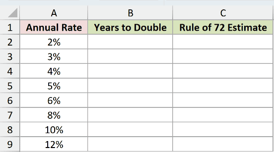
We want to find how long an amount takes to double at each annual rate.
Enter this formula in B2:
=PDURATION(A2:A9,1,2)
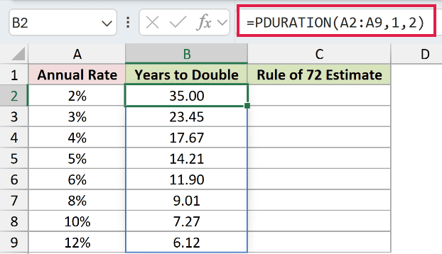
The starting and target values represent doubling. The time depends on their ratio, so the same rate produces the same doubling time regardless of the starting balance.
At 2%, PDURATION returns 35.00 years. At 8%, it returns 9.01 years.
The Rule of 72 estimates doubling time by dividing 72 by the annual rate expressed as a whole percentage. Let’s compare it with PDURATION.
Enter the comparison formula in C2:
=72/(A2:A9*100)
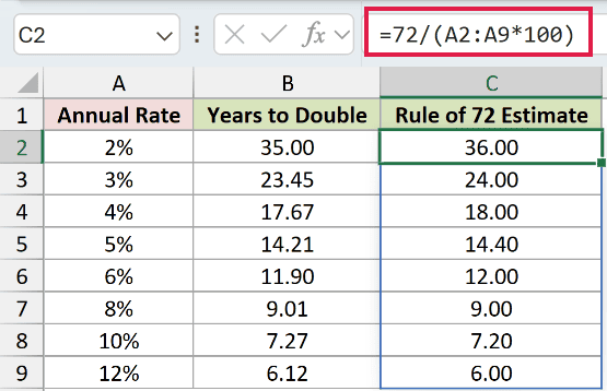
Multiplying the stored rates by 100 converts them to percentage numbers for the estimate. The formula spills into C2:C9.
At 8%, the estimate is 9.00 years, close to PDURATION’s 9.01. At 2%, the estimate is 36.00, compared with 35.00.
Use the estimate for a quick check. PDURATION calculates the compound-growth timeline directly, without relying on that shortcut.
Example 4: Round Growth Timelines to Full Months
PDURATION also works with counts that grow by a steady percentage.
Below is the dataset with channels, current subscribers, target subscribers, and monthly growth rates. Columns E and F will hold fractional and full-month timelines.
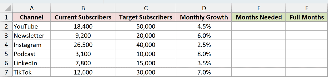
We want the months needed to reach each subscriber target, then the first full month at or beyond that timeline.
Enter this formula in E2:
=PDURATION(D2:D7,B2:B7,C2:C7)
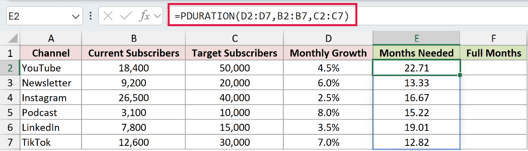
These growth rates are already monthly, so they go into PDURATION without conversion. The results spill into E2:E7.
The Newsletter row starts at 9,200 subscribers and targets 20,000 with 6.0% monthly growth. PDURATION returns 13.33 months.
For planning at month-end checkpoints, ROUNDUP rounds a positive period count upward to a whole number. That prevents PDURATION’s fractional answer from becoming an earlier checkpoint.
Enter this formula in F2:
=ROUNDUP(E2:E7,0)
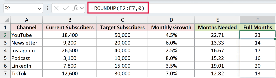
ROUNDUP requests no decimal places and spills into F2:F7. The Newsletter timeline becomes 14 full months, while the Podcast’s 15.22 months becomes 16.
Formatting a result to hide decimals doesn’t perform this upward rounding. Use the calculated Full Months values when your plan requires completed monthly periods.
Example 5: Check the Calculation Behind PDURATION
Now let’s check a single timeline against its underlying calculation.
Below is the dataset card with an annual rate in B1, current value in B2, and target value in B3. The answers will appear beside their labels.
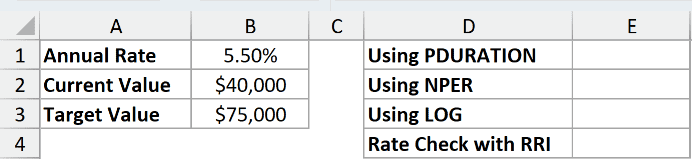
We want the years needed for $40,000 to reach $75,000 at 5.50%. Three checks verify the period count and recover the original rate.
Enter the main formula in E1:
=PDURATION(B1,B2,B3)
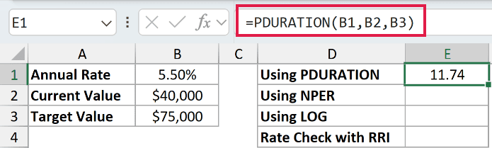
PDURATION returns 11.74 years. Both the starting and target values are positive in this formula.
NPER calculates periods for a balance with regular payments. Setting its payment argument to zero makes it comparable to PDURATION’s lump-sum calculation.
Enter that comparison in E2:
=NPER(B1,0,-B2,B3)
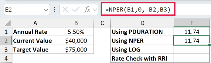
NPER also returns 11.74 years. Its starting amount is negative because the initial outflow and future inflow need opposite signs. PDURATION doesn’t use that sign convention.
LOG calculates logarithms, which let us solve for the unknown period count in compound growth. This provides a mathematical check on PDURATION.
Enter the equivalent calculation in E3:
=LOG(B3/B2)/LOG(1+B1)
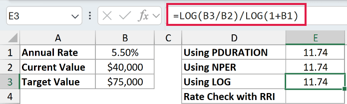
The numerator measures the target-to-starting-value ratio on a logarithmic scale. Dividing by the logarithm of the period’s growth factor returns 11.74 years again.
Finally, RRI calculates the constant growth rate connecting starting and ending values over a known period count. Feeding it PDURATION’s result checks the original rate.
Enter this formula in E4:
=RRI(E1,B2,B3)
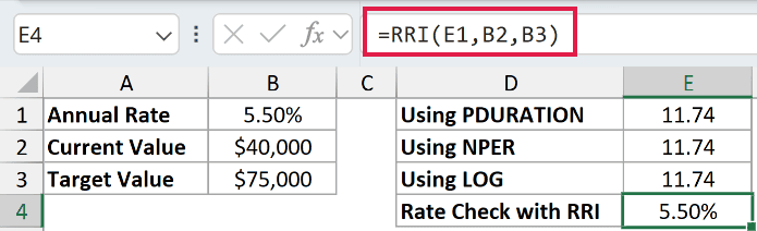
RRI returns 5.50%, matching B1. Referencing E1 uses PDURATION’s full stored result, rather than the rounded value displayed on the sheet.
Example 6: Handle Errors and Already-Reached Goals
A savings list can include goals that don’t need any more growth.
Below is the dataset with savings goals, current balances, targets, and annual rates. Columns E and F will show the raw timeline and a checked result.
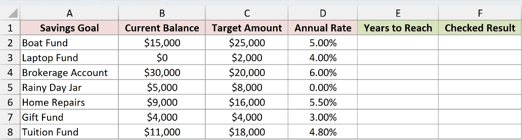
We want to identify invalid inputs and already-reached goals while keeping valid PDURATION timelines.
First, enter the raw calculation in E2:
=PDURATION(D2:D8,B2:B8,C2:C8)
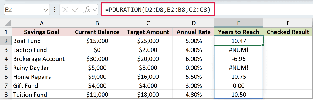
These results deliberately include errors and a negative number:
- Laptop Fund, E3:
#NUM!because its current balance is $0. Interest alone cannot grow an empty balance. - Brokerage Account, E4: -6.96 years because its $30,000 balance already exceeds the $20,000 target. This is a numeric result, not an error.
- Rainy Day Jar, E5:
#NUM!because the rate is 0.00%. - Gift Fund, E7: 0.00 years because the current balance and target are both $4,000.
IF chooses an output based on a condition. Here, it checks whether the target is already met before asking PDURATION for a timeline.
IFERROR replaces calculation errors with a message. It handles the invalid PDURATION inputs, but wouldn’t catch the negative result because that isn’t an error.
Enter the checked formula in F2:
=IF(C2:C8<=B2:B8,"Goal reached",IFERROR(PDURATION(D2:D8,B2:B8,C2:C8),"Check inputs"))
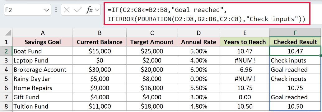
How this formula works:
- The first comparison checks whether each target is no greater than its current balance. If so, IF returns Goal reached.
- For the remaining rows, PDURATION calculates the years needed.
- IFERROR returns Check inputs when that calculation produces an error, prompting you to fix the source values.
Brokerage Account and Gift Fund now show Goal reached. Laptop Fund and Rainy Day Jar show Check inputs.
The valid results remain unchanged: 10.47 for Boat Fund, 10.75 for Home Repairs, and 10.50 for Tuition Fund.
Tips & Common Mistakes
- Match the rate to the period. Annual rates return years; monthly rates return months. Convert the rate before calculating, then convert the output only if you want another unit.
- Keep PDURATION inputs positive. A zero or negative rate, or a nonpositive starting value, returns
#NUM!. A negative timeline instead means a positive target is below the starting amount. - Enter percentage rates carefully. A rate typed as a whole number can return a plausible-looking but very short timeline without an error. Check the input’s value, not only its formatting.
- Text isn’t always rejected. Numeric text can be converted, including a rate written as
"5%". Nonnumeric text such as"abc"returns#VALUE!. - Distinguish display rounding from planning. Keep PDURATION’s stored precision for follow-up calculations. Round upward explicitly when you need the next full period, as in Example 4.
Related Excel Functions / Articles:
