
The RIGHT function in Excel returns a specified number of characters from the end of a text string.
It works well for fixed-length suffixes, such as the final digits of a code. For text after a delimiter, TEXTAFTER can avoid counting characters.
In this article, I’ll show you how to extract trailing characters, pull text after a delimiter, and convert ending digits into numbers.
RIGHT Function Syntax in Excel
Here is the syntax of the RIGHT function:
=RIGHT(text,[num_chars])
textis the text string that contains the characters you want to extract. This argument is required.[num_chars]is the number of characters to return from the end of the text. It is optional and defaults to 1.
The character count must be zero or greater. Zero returns empty text, while a count longer than the source text returns the entire source string.
RIGHT returns text, even when the extracted characters look like a number. You can use VALUE when you need a numeric result.
When to Use RIGHT Function
Use RIGHT when you need to:
- Extract a fixed-length code from the end of a text string.
- Use a different suffix length for each row.
- Return text that follows a delimiter.
- Pull trailing digits from an identifier and convert them to numbers.
- Test a final status character after removing extra spaces.
Example 1: Extract the Last Four Characters
Many tracking codes use a fixed-length suffix that carries the useful detail.
The seal codes below all end with a four-character identifier.
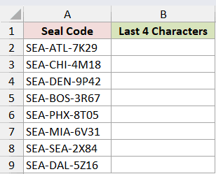
I want to extract the last four characters from every code.
Here is the formula:
=RIGHT(A2:A9,4)
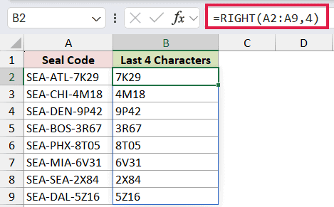
RIGHT reads four characters from the end of each value in A2:A9. The results spill into B2:B9.
For example, SEA-ATL-7K29 returns 7K29, and SEA-PHX-8T05 returns 8T05. The letters, digits, and leading zero are preserved because the result is text.
When the needed characters are not always at the end, my guide to extracting part of a text string covers other approaches.
Example 2: Use a Different Character Count for Each Row
The number of characters to extract can also come from a range.
This archive list stores the required suffix length in column B. The counts vary from one to four characters.
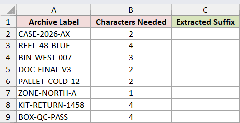
I want RIGHT to use the matching character count for each label.
Here is the formula:
=RIGHT(A2:A9,B2:B9)
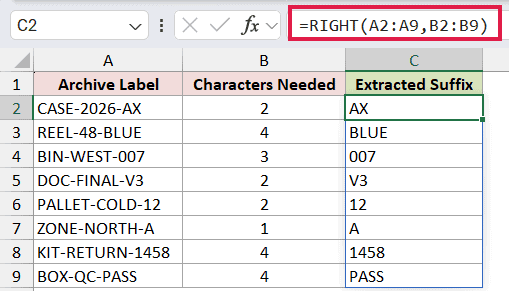
Excel pairs each label in A2:A9 with the count on the same row in B2:B9. The eight results spill into C2:C9.
CASE-2026-AX uses 2 and returns AX. REEL-48-BLUE uses 4 and returns BLUE, while ZONE-NORTH-A uses 1 and returns A.
Pro Tip: If a character count is greater than its source text length, RIGHT returns the entire text. A negative count returns #VALUE!.
Example 3: Extract Text After a Delimiter
RIGHT can work with LEN and FIND when the desired text follows a known separator.
The storage labels below place a bay name after a pipe character.
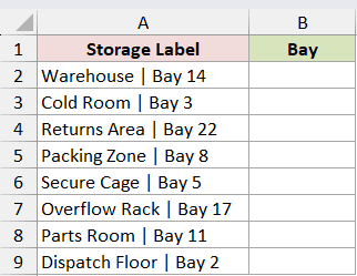
I want to return only the bay portion from each label.
Here is the formula:
=TRIM(RIGHT(A2:A9,LEN(A2:A9)-FIND("|",A2:A9)))
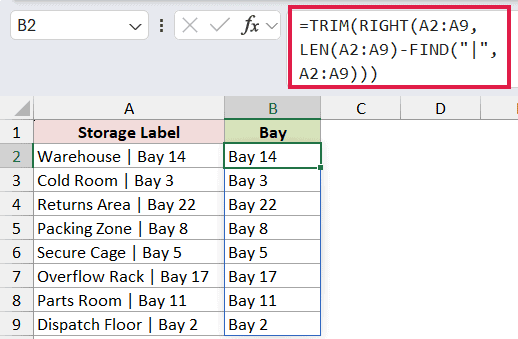
FIND locates the pipe in each text string. LEN minus that position calculates how many characters remain, and RIGHT extracts them.
TRIM removes the space immediately after the pipe delimiter. The first warehouse entry therefore returns Bay 14, and the dispatch-floor entry returns Bay 2.
The FIND function is case-sensitive, though that does not matter for the pipe used here. In Microsoft 365 and Excel 2024, the simpler modern alternative is =TEXTAFTER(A2:A9,"|").
Example 4: Convert Trailing Digits to Numbers
RIGHT always returns text, but you can wrap it in VALUE when the extracted digits need to behave as numbers.
This meter log uses identifiers that all end with a three-digit reading.
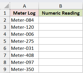
I want to extract each reading and convert it to a numeric value.
Here is the formula:
=VALUE(RIGHT(A2:A9,3))
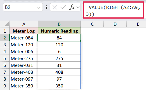
RIGHT first returns the final three characters. VALUE then converts those text digits into numbers, and the results spill into B2:B9.
Meter-084 becomes 84, Meter-006 becomes 6, and Meter-350 becomes 350. Numeric conversion removes leading zeros, which is useful for calculations but not for codes that must retain their original width.
For strings where digits may appear at the beginning or middle, use one of the broader methods for extracting numbers from text.
Example 5: Handle Trailing Spaces
Trailing spaces can make RIGHT return a blank character instead of the status code you expect.
The inspection tags below end in R or A, but several values have one or two spaces after the code.
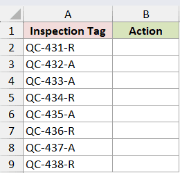
I want to label R tags for review and release the A tags.
Here is the formula:
=IF(RIGHT(TRIM(A2:A9))="R","Review","Release")
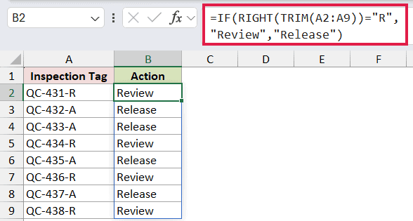
The TRIM function removes ordinary extra spaces before RIGHT reads the final character. RIGHT omits num_chars, so it returns one character by default.
The IF function returns Review when that character is R. Otherwise, it returns Release. The final results alternate correctly even though the original tags have inconsistent trailing spaces.
This formula assumes every cleaned tag ends in R or A. If other codes are possible, add an explicit test for A rather than treating every non-R value as Release.
Tips & Common Mistakes
- Omit
num_charsonly when you want the final single character. RIGHT uses 1 by default. - Use zero or a positive character count. A negative count returns #VALUE!.
- RIGHT returns all the source text when
num_charsis longer than the text. - Remember that numeric-looking output is still text. Wrap RIGHT in VALUE when you need to calculate with the extracted digits.
- Keep the spill area empty in current Excel. A blocked result range causes a #SPILL! error.
- Use TEXTAFTER for delimiter-based extraction in Microsoft 365 or Excel 2024. It is clearer and can target a specific delimiter occurrence.
- TRIM removes ordinary spaces but not every nonprinting or nonbreaking character commonly found in imported data.
I covered fixed and variable suffixes, delimiter-based extraction, numeric conversion, and trailing spaces. I hope you found this article helpful.
Related Excel Functions / Articles:
