
The SEARCHB function in Excel returns the starting position of text within another text string, ignoring uppercase and lowercase differences.
That position helps you locate a label or extract the text beside it. SEARCHB also accepts wildcards, so your search can allow gaps or changing characters.
In this article, I’ll show you how to match text regardless of case, search with wildcards, and skip a prefix before locating a match.
SEARCHB Function Syntax in Excel
SEARCHB takes the text to find, the text to search, and an optional starting position.
=SEARCHB(find_text, within_text, [start_num])
- find_text (required): The text or wildcard pattern you’re looking for. Put typed text in double quotes.
- within_text (required): The text to search, supplied directly or through a cell reference or range.
- start_num (optional): Where the search begins. If omitted, SEARCHB starts at the beginning. Its result still measures the match’s position from the beginning of the original text.
Microsoft marks SEARCHB as deprecated, although it still calculates.
When to Use SEARCHB Function
- Locate text in an existing SEARCHB workbook when capitalization varies between entries.
- Find a pattern within report titles that don’t share a consistent separator.
- Check whether terms appear in a particular order within notes.
- Locate a label after a fixed prefix, then use its position to extract nearby text.
Example 1: Find Text Regardless of Case
Let’s start with maintenance notes whose capitalization varies.
Below is the dataset. Column A contains work order notes, while columns B and C will hold the search positions and a case-sensitive comparison.
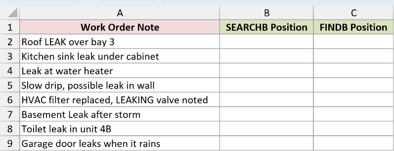
We want to locate “leak” in each note, regardless of how someone capitalized it.
Enter this formula in B2:
=SEARCHB("leak",A2:A9)
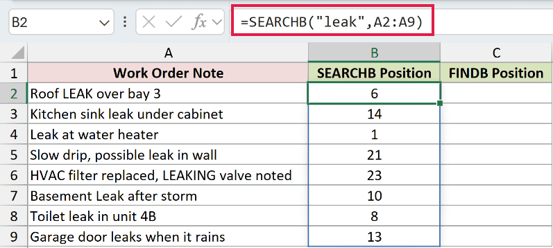
The formula spills its results into B2:B9. “Roof LEAK over bay 3” returns 6, while “Leak at water heater” returns 1.
SEARCHB also finds text inside a longer word. The note containing “LEAKING” returns 23, so this isn’t a whole-word test.
Range formulas spill in Excel 2021, Excel 2024, and Microsoft 365. In Excel 2019 and earlier, use a per-row reference and copy down.
For comparison, FINDB locates text with matching capitalization.
Enter the comparison formula in C2:
=FINDB("leak",A2:A9)
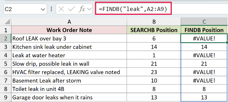
The comparison returns #VALUE! in C2, C4, C6, and C7 because their capitalization doesn’t match lowercase “leak”. These errors are deliberate.
For “Kitchen sink leak under cabinet”, both columns return 14. Here, the note already contains the exact lowercase text.
Example 2: Find a Year With Question Marks
Report titles don’t always put the year after the same separator.
Below is the dataset. Column A contains report titles with varied punctuation and spacing, and column B will hold the extracted year.
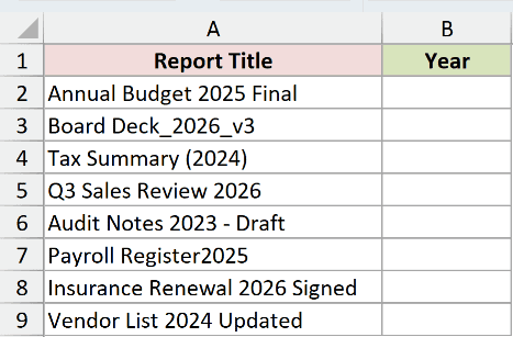
We want SEARCHB to locate the year pattern, then extract the matching text.
MIDB extracts text from a starting byte position. Here, it uses the position returned by SEARCHB to pick out the year.
Enter this formula in B2:
=MIDB(A2:A9,SEARCHB("20??",A2:A9),4)
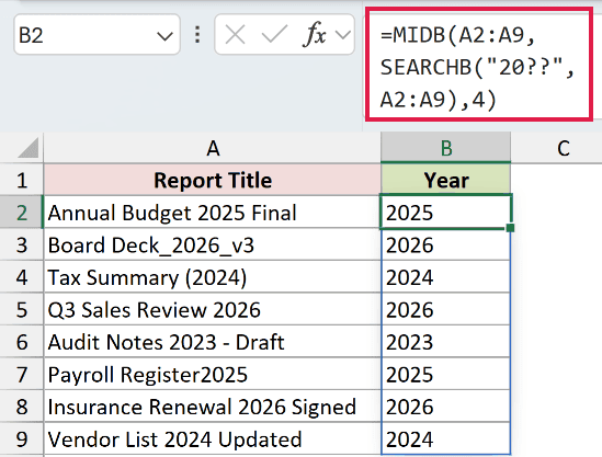
The pattern 20?? means the literal text “20” followed by a character for each question mark. MIDB extracts the matched year, and the results spill down.
“Annual Budget 2025 Final” returns 2025, while “Tax Summary (2024)” returns 2024. These extracted results are text.
“Payroll Register2025” also returns 2025. SEARCHB finds the pattern even when no space separates it from the preceding word.
Pro Tip: A question mark matches any character, including letters and digits. Check that the extracted text is a year before using it.
Example 3: Match Words Across a Gap
An asterisk lets SEARCHB match text with a changing gap between terms.
Below is the dataset. Columns A and B contain account IDs and billing notes. Columns C and D will hold match positions and TRUE/FALSE flags.
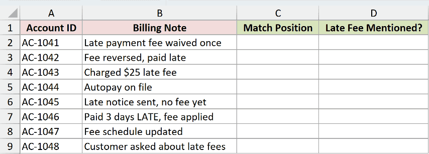
We want to find notes containing “late” followed somewhere by “fee”.
Enter this formula in C2:
=SEARCHB("late*fee",B2:B9)
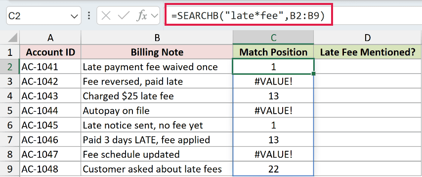
The asterisk allows intervening text. “Late payment fee waived once” returns 1, while “Customer asked about late fees” returns 22.
“Fee reversed, paid late” returns #VALUE! because the terms appear in the wrong order. “Autopay on file” and “Fee schedule updated” also return #VALUE!.
To turn these positions into flags, ISNUMBER checks whether SEARCHB returned a number. A successful match becomes TRUE; an unsuccessful search becomes FALSE.
Enter this formula in D2:
=ISNUMBER(SEARCHB("late*fee",B2:B9))
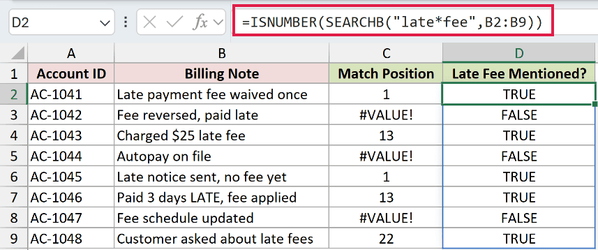
The flags spill down column D. “Late payment fee waived once” returns TRUE, while “Fee reversed, paid late” returns FALSE.
Pro Tip: “Late notice sent, no fee yet” returns TRUE in the flag column. Review flagged notes to confirm whether a fee was charged.
Example 4: Find an Actual Asterisk
A footnote asterisk needs a different search pattern from a wildcard.
Below is the dataset. Column A lists membership plans. Columns B and C will compare a bare asterisk search with an escaped asterisk search.
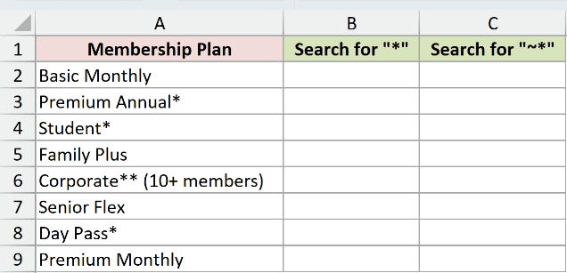
We want to locate actual footnote markers in the plan names.
For the correct literal search, enter this formula in C2:
=SEARCHB("~*",A2:A9)
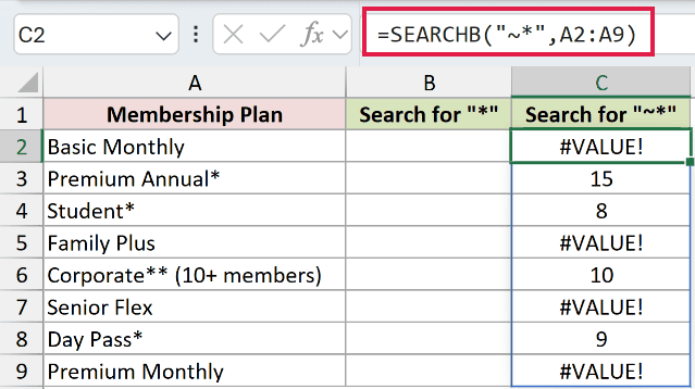
The tilde tells SEARCHB to treat the asterisk as a literal character. “Premium Annual” returns 15, “Student” returns 8, and “Day Pass*” returns 9.
Corporate** (10+ members) returns 10, the position of its first asterisk.
C2, C5, C7, and C9 deliberately show #VALUE!. Those plan names don’t contain an asterisk.
Now enter this comparison in B2 to see the mistake of searching with an unescaped asterisk:
=SEARCHB("*",A2:A9)
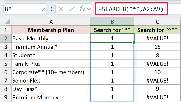
The mistaken formula returns 1 for every plan, including “Basic Monthly”. Its asterisk is a wildcard, so it doesn’t test for a printed footnote marker.
Example 5: Skip a Timestamp Before Searching
Log entries can contain the same punctuation in a timestamp and a message label.
Below is the dataset. Column A contains log entries. Columns B and C will compare the first colon with the colon after the timestamp.
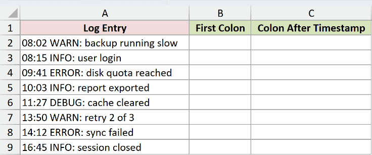
We want the colon after the log level, such as WARN or ERROR.
Enter this formula in C2 to start searching beyond the timestamp:
=SEARCHB(":",A2:A9,7)
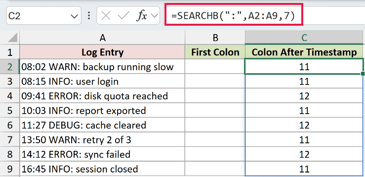
Starting at position 7 skips the timestamp’s colon. “08:02 WARN: backup running slow” returns 11, while “09:41 ERROR: disk quota reached” returns 12.
The answer still counts from the beginning of the entire entry.
For comparison, enter this formula in B2 without a starting position:
=SEARCHB(":",A2:A9)
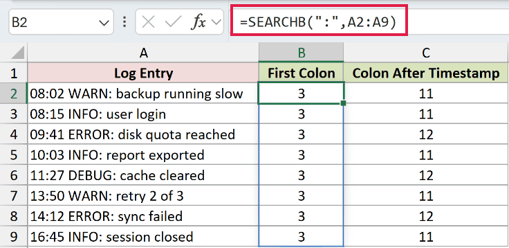
This comparison returns 3 throughout B2:B9 because it finds the timestamp’s colon. That’s the wrong delimiter for our task.
Example 6: Extract After a Case-Varying Label
Bank descriptions may use the same reference label with different capitalization and spacing.
Below is the dataset. Column A contains transaction descriptions, and column B will hold the extracted reference numbers.
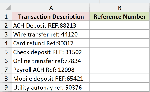
We want to extract the reference after “ref:”, regardless of capitalization or a space after the colon.
MIDB extracts text after SEARCHB locates the label. TRIM removes surrounding spaces from that extracted text, handling descriptions with a space after the colon.
Enter this formula in B2:
=TRIM(MIDB(A2:A9,SEARCHB("ref:",A2:A9)+4,20))
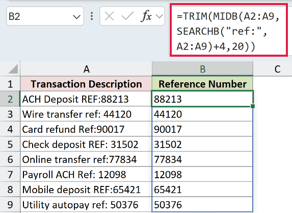
How this formula works:
- SEARCHB locates
ref:even when the description usesREF:orRef:. - The addition moves the starting position past the complete label, including its colon.
- The
20tells MIDB to extract up to20bytes from the position SEARCHB found plus the label length. These descriptions end with the reference. - TRIM removes the extra leading space where present, and the results spill into B2:B9.
“ACH Deposit REF:88213” returns 88213, and “Wire transfer ref: 44120” returns 44120. Both results are text.
“Card refund Ref:90017” returns 90017. Including the colon in the search text prevents SEARCHB from confusing the label with the earlier word “refund”.
Pro Tip: The reference must end the description. Any note after it can enter the extracted result, so check your export’s format before reusing this formula.
Tips & Common Mistakes
- SEARCH finds text using character positions. SEARCHB matches it unless your default editing language is a double-byte language (Japanese, Chinese, Korean).
- A missing match returns
#VALUE!. Check both the search text andstart_numbefore treating the error as a data problem. - A starting position of zero or beyond the text’s length returns
#VALUE!. Starting after the only match also leaves nothing to find. - Use
~?to search for a literal question mark and~~to search for a literal tilde. The escaping rule works like the asterisk example. - An empty search string can return a position. Check that a search-input cell actually contains the text you intended to find.
Related Excel Functions / Articles:
