
Excel’s TRUNC function removes digits beyond a specified position without rounding the number.
It is useful when extra decimal places should be discarded rather than rounded. With no digit count supplied, TRUNC removes the fractional part and keeps the integer portion.
For negative numbers, that moves the result toward zero. INT instead rounds down to the next lower integer.
In this article, I’ll show you how to remove decimal places without rounding, compare negative results with INT, and remove time from date values.
TRUNC Function Syntax in Excel
The TRUNC function accepts a number and lets you choose where Excel cuts off its remaining digits.
=TRUNC(number, [num_digits])
- number (required) is the number or cell reference you want to truncate.
- num_digits (optional) controls how many decimal places remain. It defaults to 0 when omitted.
When to Use TRUNC Function
- Remove the fractional part of numbers without rounding them.
- Keep a fixed number of decimal places while discarding later digits.
- Cut large positive numbers at the tens, hundreds, thousands, or another place.
- Compare toward-zero truncation with the INT function on negative numbers.
- Separate a positive number into whole and fractional parts.
- Remove the time portion from Excel date and time values.
Example 1: Remove Decimals From Trip Distances
Let’s start with trip distances that need clean whole-mile values.
Below is the dataset. Column A lists eight trip IDs, and column B contains each trip distance in miles.
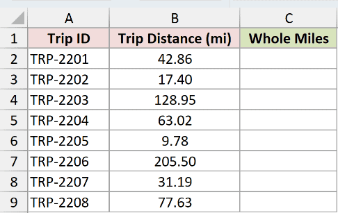
We want one TRUNC formula to remove each fractional mile and spill the whole-mile results down column C.
Here is the formula:
=TRUNC(B2:B9)
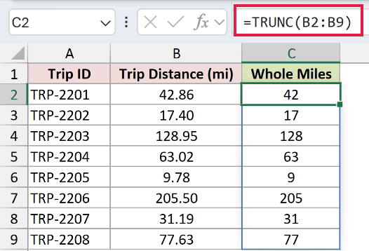
The formula omits num_digits, so Excel uses its default of 0. It returns 42 for 42.86 and 205 for 205.50.
TRUNC removes the decimal portion without checking whether the next digit would normally cause rounding.
Pro Tip: TRUNC changes the stored number. A zero-decimal number format only changes what you see, so later calculations still use the hidden decimal portion.
Example 2: Keep Four Decimals Without Rounding
Now let’s keep four decimal places in a set of market exchange rates.
Below is the dataset. Column A identifies eight currency pairs, and column B contains each market rate to six decimal places.
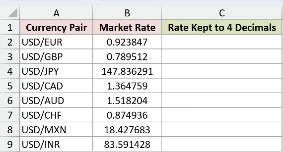
We want to retain four decimal places for every rate without rounding the final retained digit.
Here is the formula:
=TRUNC(B2:B9,4)
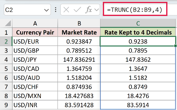
The num_digits argument is 4, so the spilled results keep four decimal places. The USD/JPY rate changes from 147.836291 to 147.8362.
Every later digit is discarded. None of those digits can increase the fourth decimal place, which is what separates truncation from rounding.
Use ROUND instead when you want the next digit to determine whether the final retained digit changes.
Example 3: Truncate Numbers to Thousands
Here’s how TRUNC handles digits to the left of the decimal point.
Below is the dataset. Column A lists eight metro areas, and column B contains their population estimates.
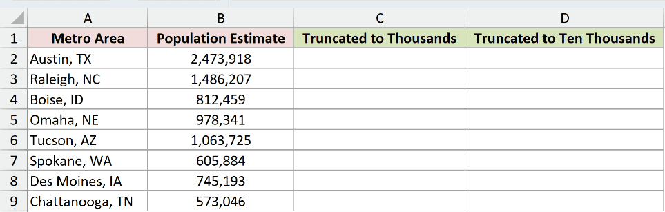
We want separate spilled views truncated to the thousands and ten-thousands places.
Here is the formula that cuts each estimate at the thousands place:
=TRUNC(B2:B9,-3)
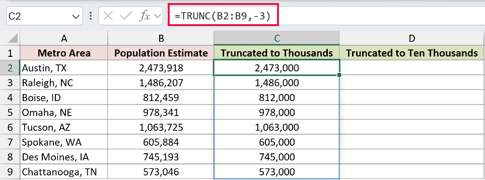
And here is the formula that cuts each estimate at the ten-thousands place:
=TRUNC(B2:B9,-4)
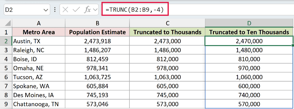
A negative num_digits value moves the cut point left of the decimal. The first formula removes everything below thousands, while the second removes everything below ten thousands.
For Austin, 2,473,918 becomes 2,473,000 in column C and 2,470,000 in column D.
TRUNC still does not round here. It keeps the digits before the chosen cut point and replaces the remaining positions with zeros.
Example 4: Compare TRUNC and INT on Negatives
Now let’s look at the difference that matters most with negative numbers.
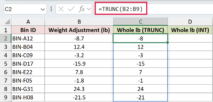
Below is the dataset. Column A lists eight bin IDs, and column B contains positive and negative weight adjustments.
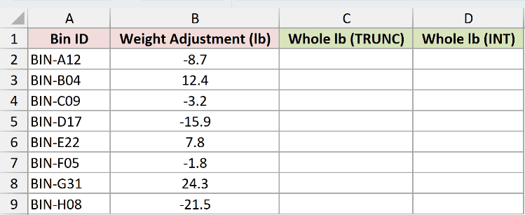
We want to truncate every adjustment first, then compare those results with INT.
Here is the TRUNC formula:
=TRUNC(B2:B9)
And here is the INT formula for comparison:
=INT(B2:B9)
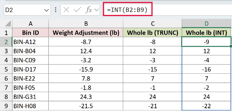
TRUNC moves toward zero, while INT rounds down to the next lower integer. For BIN-A12, -8.7 becomes -8 with TRUNC and -9 with INT.
Positive values match in both columns. The difference appears only on negative numbers, which is why this dataset includes several negative adjustments.
Example 5: Split Whole and Fractional Parts
Let’s use TRUNC to separate fuel amounts into two useful pieces.
Below is the dataset. Column A identifies eight vehicles, and column B contains the gallons pumped for each one.
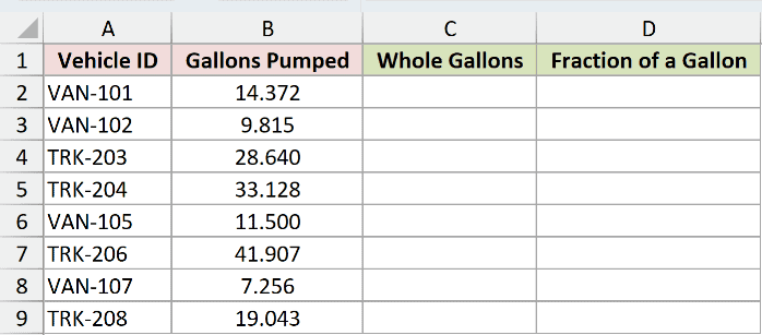
We want one spilled column for whole gallons and another for the remaining fraction.
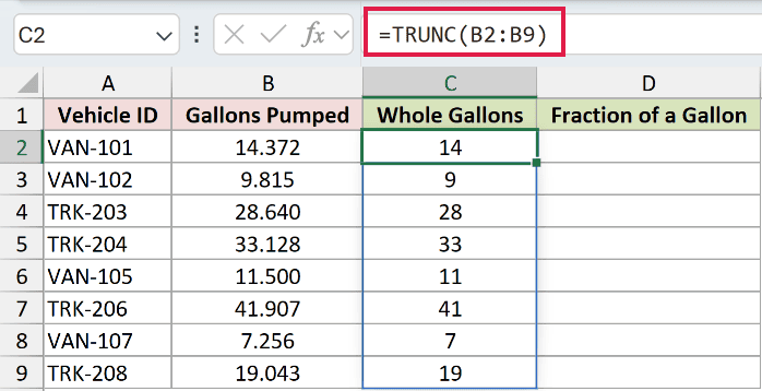
Here is the formula for the whole gallons:
=TRUNC(B2:B9)
And here is the formula for the fractional remainder:
=B2:B9-TRUNC(B2:B9)
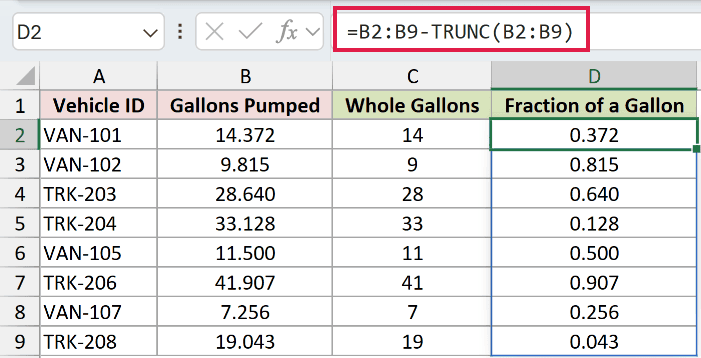
The first formula removes each fractional portion. The second subtracts those whole gallons from the original amounts.
For VAN-101, 14.372 splits into 14 and 0.372. For TRK-203, 28.640 splits into 28 and 0.640.
MOD can also return the fractional part of positive numbers. The sign differs with negative values, so this subtraction method preserves the original fraction’s sign.
Example 6: Remove Time From Date Values
Finally, let’s strip the time from a column of order timestamps.
Below is the dataset. Column A lists eight order IDs, and column B contains the date and time when each order was placed.
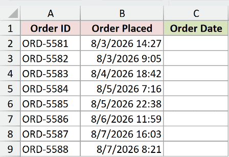
We want to remove every time portion and spill the corresponding dates down column C.
Here is the formula:
=TRUNC(B2:B9)
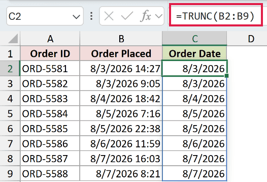
Excel stores a date and time as a positive serial number. The whole part represents the date, while the fractional part represents the time.
TRUNC removes that fraction, so 8/3/2026 14:27 becomes 8/3/2026. The result column uses a date format to display the remaining whole value correctly.
INT gives the same result for these positive date serials.
Tips & Common Mistakes
- TRUNC never rounds up or down. It removes digits beyond the chosen cut point and leaves the retained digits unchanged.
- Omit num_digits when you only need the integer portion. Writing 0 explicitly can make the formula’s intent clearer in a shared workbook.
- Treat negative num_digits as a place-value control for reporting bands such as thousands, rather than as decimal precision.
- ROUNDDOWN returns the same result as TRUNC for every input, including negative numbers. The only difference is that TRUNC lets you omit num_digits, while ROUNDDOWN requires it.
- Clear any occupied cells in the intended spill range when Excel returns #SPILL!. One blocked cell prevents the entire result column from appearing.
- An implicit intersection operator before TRUNC forces a single result. Remove that operator when you want a range argument to spill.
- In Excel 2019 and earlier, enter a row-level TRUNC formula and fill it down, or use a legacy array formula for the selected result range.
- TRUNC treats a referenced blank cell as 0, which can hide missing inputs. Check for blanks first when an empty cell should remain empty.
- TRUNC coerces text that looks numeric, but genuinely nonnumeric text returns #VALUE!. Check imported columns when truncation fails after a CSV import.
- Use a TRUNC result, not cell formatting, when later formulas must ignore the discarded digits.
Revisit the market-rate example for decimals, the population example for place values, or the order example for timestamps.
For negative numbers with decimals, remember that TRUNC moves toward zero while INT moves to the next lower integer.
Related Excel Functions / Articles:
