
Excel’s INT function rounds a number down to the nearest integer.
For positive numbers, that removes the decimal portion. Negative numbers move toward the next lower integer, which is why INT and TRUNC can return different results.
In this article, I’ll show you how to handle negative-number rounding, separate dates from times, and split minutes into hours and remaining minutes.
INT Function Syntax in Excel
The INT function needs only the number you want to round down.
=INT(number)
- number (required) is the number, cell reference, or range you want to round down to the nearest integer.
When to Use INT Function
- Remove the decimal portion from positive numbers while rounding down.
- Round negative numbers toward the next lower integer.
- Remove the time portion from Excel date-time values.
- Calculate completed units, such as years or hours.
- Separate whole dollars from the cents in an amount.
Example 1: Round a Column Down to Whole Numbers
Let’s start with the basic rounding-down job.
Below is the dataset. Column A lists pet supplies, and column B contains their shelf weights in pounds.
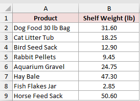
We want one formula to round every shelf weight down to a whole number.
Here is the formula:
=INT(B2:B9)
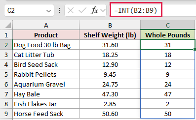
The range B2:B9 makes INT return eight results. Excel places them in column C from the single formula entered in C2.
For example, 31.60 becomes 31, while 2.85 becomes 2.
TRUNC and ROUNDDOWN with zero digits give the same results for these positive values. INT is shorter when rounding down to an integer is all you need.
Pro Tip: Keep C2:C9 empty before entering the formula. Any value in the spill area causes a #SPILL! error.
Example 2: Compare INT and TRUNC With Negatives
Negative numbers are where INT often catches people out.
Below is the dataset. Column A lists freezer units, and column B contains their temperature readings.
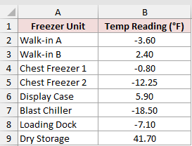
We want to see how both functions handle the same positive and negative readings.
Here is the INT formula:
=INT(B2:B9)
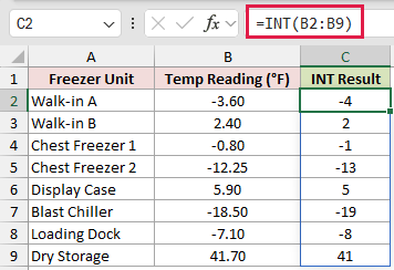
To show how INT differs from truncation for negatives, here is the TRUNC formula:
=TRUNC(B2:B9)
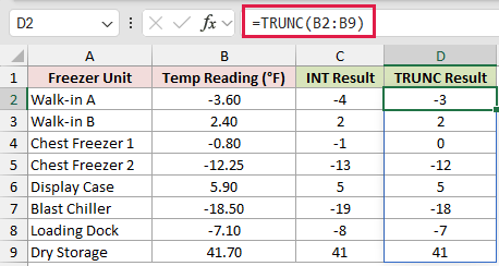
INT rounds toward negative infinity. It changes -3.60 to -4, -0.80 to -1, and -12.25 to -13.
TRUNC removes the decimal portion and moves toward zero. The same three readings become -3, 0, and -12.
For positive readings, both functions return the same integer. For example, both change 5.90 to 5.
Pro Tip: ROUNDDOWN with zero digits behaves like TRUNC for negative numbers. FLOOR.MATH with its default settings behaves like INT.
Example 3: Separate a Date and Time
Here’s a handy way to split appointment timestamps into separate date and time values.
Below is the dataset. Column A contains each appointment timestamp.
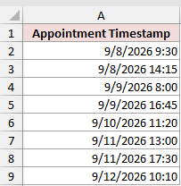
We want to extract both parts of every timestamp with two spilling formulas.
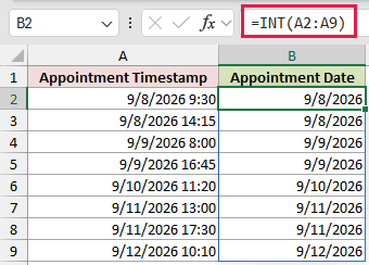
Here is the formula for the date:
=INT(A2:A9)
And here is the formula for the time:
=A2:A9-INT(A2:A9)
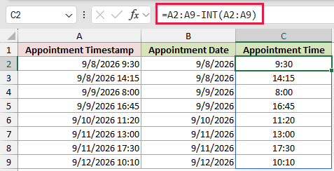
Excel stores a date as a whole number and time as a fraction of a day. INT keeps the whole-number date serial and removes the time fraction.
Subtracting that whole number from the original timestamp leaves only the time. The first row returns 9/8/2026 and 9:30.
You can also get the time portion with =MOD(A2:A9,1). The subtraction version makes the split between the whole and fractional parts visible.
Pro Tip: Apply a date format to column B and a time format such as h:mm to column C. Otherwise, Excel may display serial numbers or decimals.
Example 4: Calculate Age in Completed Years
Here’s how to calculate each employee’s age on a fixed date.
Below is the dataset. Column A lists employees, column B contains birth dates, and E2 holds the as-of date of 9/1/2026.
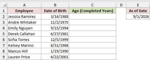
We want to calculate each employee’s completed age as of the date in E2.
Enter this formula in C2, then copy it down through C9:
=INT(YEARFRAC(B2,$E$2))
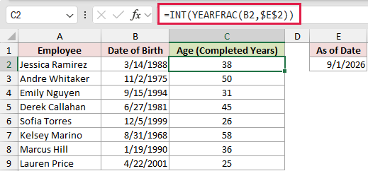
YEARFRAC calculates the years between the birth date in B2 and the fixed date in E2. INT removes the unfinished fraction of the current year.
The absolute reference $E$2 keeps the as-of date unchanged as the formula is copied down. The completed ages range from 25 to 58.
This example uses a fill-down formula because YEARFRAC does not spill across the source range. INT itself still supports spilling when given a compatible range.
DATEDIF can return completed years directly with =DATEDIF(B2,$E$2,"y"). With INT and YEARFRAC, you can see the fractional-year step before INT removes it.
Example 5: Split Minutes Into Hours and Minutes
Now let’s turn total task minutes into a more readable duration.
Below is the dataset. Column A lists tasks, and column B contains the minutes logged for each one.
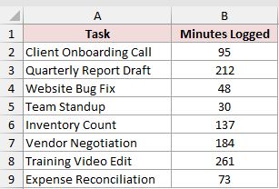
We want to split every duration into whole hours and remaining minutes.
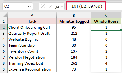
Here is the formula for whole hours:
=INT(B2:B9/60)
And here is the formula for leftover minutes:
=MOD(B2:B9,60)
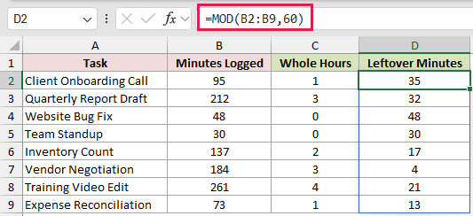
Dividing by 60 converts minutes to hours. INT keeps only the completed hours, while MOD returns the remainder after division by 60.
The 212-minute report becomes 3 hours and 32 minutes. The 261-minute video edit becomes 4 hours and 21 minutes.
QUOTIENT can calculate the whole hours directly with =QUOTIENT(B2:B9,60). The INT version remains useful when you already think of the calculation as decimal hours.
Example 6: Split Amounts Into Dollars and Cents
Our last example separates invoice amounts into whole dollars and cents.
Below is the dataset. Column A lists invoice numbers, and column B contains the corresponding amounts.
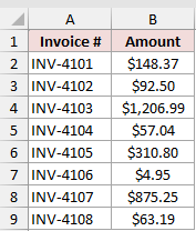
We want to split every positive amount into separate whole-dollar and cent values.
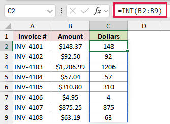
Here is the formula for dollars:
=INT(B2:B9)
And here is the formula for cents:
=ROUND((B2:B9-INT(B2:B9))*100,0)
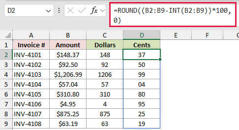
INT returns the whole-dollar portion. Subtracting it from the amount leaves the decimal fraction, which the formula multiplies by 100 to get cents.
ROUND removes tiny floating-point differences that can appear in decimal arithmetic. For example, $148.37 becomes 148 dollars and 37 cents.
The $92.50 invoice becomes 92 dollars and 50 cents. The two-digit number format keeps that cent value displayed as 50.
Pro Tip: This setup assumes positive amounts. Test refunds or other negative values separately because INT rounds them toward the next lower integer.
Tips & Common Mistakes
- INT always rounds down. With negative numbers, that means moving away from zero, so
=INT(-3.6)returns -4. - TRUNC and
ROUNDDOWN(number,0)move negative values toward zero. Use them when you want to remove decimals instead of flooring the number. - In Excel 365 and newer dynamic-array versions, a range-based INT formula spills automatically. Blocked output cells cause #SPILL!.
- Adding
@before INT applies implicit intersection and forces a single result instead of a spill. - In older Excel versions, enter INT with one cell reference and copy the formula down. A legacy Ctrl+Shift+Enter array formula is possible but usually less convenient.
- Format INT results to match their meaning. Date serials need a date format, while ordinary rounded values usually need a zero-decimal number format.
INT always moves to the next lower whole number.
That direction matters most when your source values can be negative.
Related Excel Functions / Articles:
