
Excel’s UNICODE function returns the decimal Unicode code point for the first character in a text value.
That number helps identify hidden spaces, inconsistent punctuation, and symbols that look similar on screen. To inspect another position, first isolate that character with a text function.
In this article, I’ll show you how to inspect character codes, find hidden nonbreaking spaces, and identify inconsistent separators with UNICODE.
UNICODE Function Syntax in Excel
The UNICODE function uses the following syntax:
=UNICODE(text)
textis the text value or cell reference whose first character you want to inspect.
When to Use UNICODE Function
- Identify the first character in imported text.
- Distinguish ordinary spaces from nonbreaking spaces.
- Check whether labels begin with uppercase letters, lowercase letters, numbers, or symbols.
- Diagnose similar-looking punctuation in codes and identifiers.
- Return one character code for every value in a range.
Example 1: Check Different Character Positions
Let’s begin with one text value and inspect two positions.
Below is a small dataset containing the text “Apex Supplies” in cell A2.

The first check is the Unicode code point for the opening letter in A2.
Here is the formula:
=UNICODE(A2)
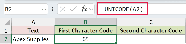
The formula returns 65, the Unicode code point for uppercase A. UNICODE reads only the first character of the supplied text.
The next check is the code point for the second character.
Here is the formula:
=UNICODE(MID(A2,2,1))
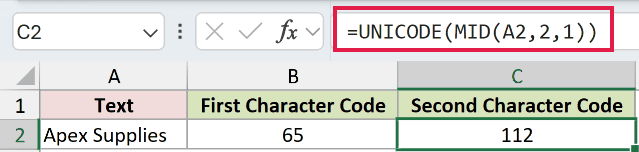
The MID function extracts one character beginning at position 2, which is the lowercase p. UNICODE then returns 112 for that extracted character.
Pro Tip: UNICODE always inspects the first character of its text argument. Use MID or RIGHT when the character you need is elsewhere.
Example 2: Spill Unicode Codes for a Range
Modern Excel can inspect a complete range with one formula.
Below is an imported-label dataset in A2:A8 containing uppercase text, lowercase text, text beginning with a digit, the euro sign, and a check mark.
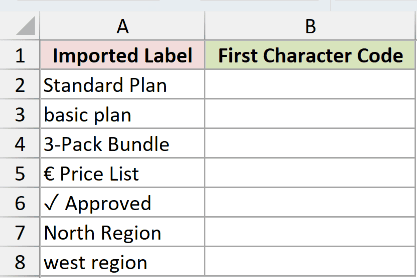
The result should show one first-character code beside every imported label.
Here is the formula:
=UNICODE(A2:A8)
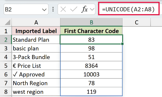
The single formula in B2 spills seven results through B8. For example, Standard Plan returns 83, basic plan returns 98, and 3-Pack Bundle returns 51.
The euro sign returns 8364, while the check mark returns 10003. These values show why a Unicode-aware function is useful beyond basic letters and numbers.
Pro Tip: Range input spills in Microsoft 365, Excel 2024, Excel 2021, and Excel for the web. In Excel 2019 or 2016, use a single-cell formula and fill it down.
Example 3: Find and Remove Nonbreaking Spaces
UNICODE can expose a hidden character before you clean it.
Below is an imported-contact dataset in A2:A9. Some names begin with an ordinary space, some with a nonbreaking space, and others have no leading space.
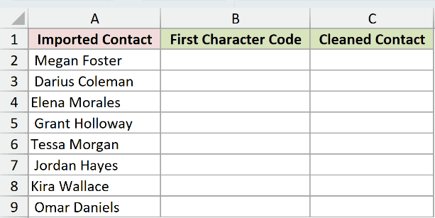
The first step is to identify the opening character in every contact name.
Here is the formula:
=UNICODE(A2:A9)
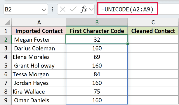
The result distinguishes three cases. An ordinary leading space returns 32, a nonbreaking space returns 160, and a name beginning with a letter returns that letter’s code.
After identifying those spaces, I want to remove them and clean all eight names.
Here is the formula:
=TRIM(SUBSTITUTE(A2:A9,UNICHAR(160)," "))
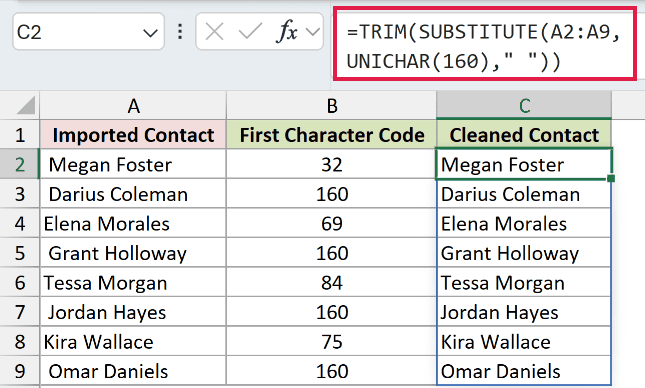
How this formula works:
- The UNICHAR function returns the nonbreaking-space character identified by UNICODE.
- The SUBSTITUTE function replaces every character 160 with an ordinary space.
- The TRIM function removes the resulting leading spaces and returns the cleaned contact names in C2:C9.
TRIM alone does not remove character 160. Replacing it first is what makes the cleanup work.
Pro Tip: Diagnose the character before replacing it. A visually blank character could be an ordinary space, a nonbreaking space, or another Unicode character.
Example 4: Identify Inconsistent Code Separators
The same approach works for punctuation inside a text string.
Below is an imported-code dataset in A2:A8. Some work-order codes use a hyphen, while others use the similar-looking en dash character.
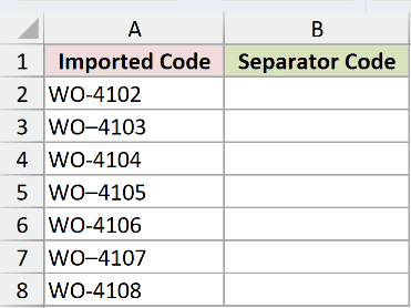
The goal is to inspect the separator in the third position of every code.
Here is the formula:
=UNICODE(MID(A2:A8,3,1))
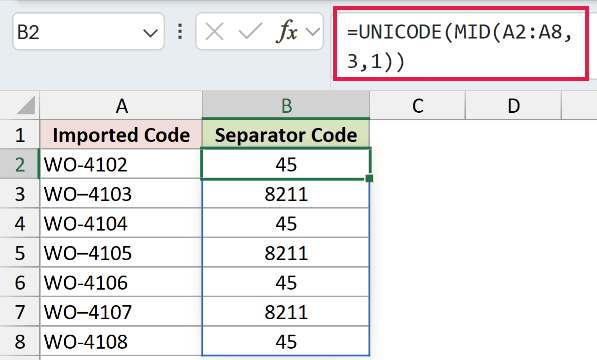
MID extracts the third character from each code. UNICODE returns 45 for the hyphen and 8211 for the en dash.
The different numbers make the inconsistent separators easy to flag, even when the characters look almost identical in the worksheet.
Tips & Common Mistakes
- UNICODE reads the first character only. Use a text function such as MID to pass a different character into it.
- UNICHAR performs the reverse conversion. It returns the character represented by a Unicode number.
- The CODE function returns a number from the computer’s character set. Use UNICODE when you need code points covering a wider range of characters.
- Invalid text data or a partial surrogate can return
#VALUE!. - Format result cells as numbers so Excel displays the code points as integers.
- The UNICODE function is available in Microsoft 365, Excel 2024, Excel 2021, Excel 2019, and Excel 2016.
- Range formulas spill only in dynamic-array versions. Older versions need a single-cell formula copied down.
I covered how to inspect first and later characters, spill codes for a range, and diagnose hidden spaces or inconsistent separators.
I hope you found this article helpful.
Related Excel Functions / Articles:
