ACCRINTM Function in Excel (4 Easy Examples)

The ACCRINTM function in Excel returns accrued interest for a security that pays its interest at maturity.

It uses the issue date, maturity date, annual coupon rate, face amount, and day-count basis. Unlike ACCRINT, it is meant for a single payment at maturity.

In this article, I’ll show you how to calculate a security register, use the default par value, compare day-count bases, and find maturity proceeds.

Table of Contents

ACCRINTM Function Syntax in Excel

The ACCRINTM function uses four required arguments and one optional argument:

=ACCRINTM(issue, settlement, rate, par, [basis])

issue is the security’s issue date.
settlement is the maturity date, when the security pays its interest.
rate is the annual coupon rate.
par is the security’s face amount. Microsoft documents a $1,000 default when this argument is omitted.
basis is the optional day-count basis. Use 0 or omit it for US 30/360, 1 for Actual/Actual, 2 for Actual/360, 3 for Actual/365, or 4 for European 30/360.

When to Use ACCRINTM Function

Calculate interest on a security that pays all interest at maturity.
Process a register containing securities with different rates, dates, face amounts, or bases.
Compare results under different day-count conventions.
Add accrued interest to principal to find the amount received at maturity.

Example 1: Calculate Interest for Several Securities

Let’s start with a small register of maturity-only securities.

Below are six securities with their issue dates, maturity dates, coupon rates, face amounts, and basis codes. The Accrued Interest column is ready for formulas.

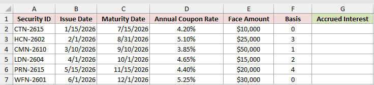
I want to calculate the accrued interest for every security.

Enter this formula in G2, then fill it down through G7:

=ACCRINTM(B2,C2,D2,E2,F2)

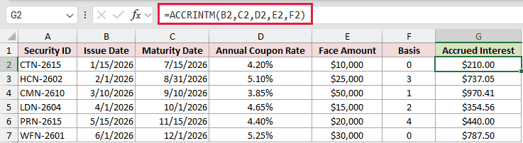
Each row passes one security’s inputs to ACCRINTM. For example, the first row returns $210.00, while the second returns $737.05.

The relative references change as you fill the formula down. Native Excel returned #VALUE! when these inputs were passed as plain ranges, so this example uses scalar formulas.

Pro Tip: Enter rates as percentages or decimal values. A typed value of 4.2 means 420%, while 4.2% means 0.042.

Example 2: Use ACCRINTM’s Default Par Value

Excel can use a $1,000 par value when you leave the fourth argument empty.

Below is a parameter card with an issue date, maturity date, coupon rate, and an empty accrued-interest result cell.

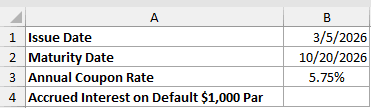
I want to calculate interest without entering a separate face amount or basis.

Here is the formula:

=ACCRINTM(B1,B2,B3,)

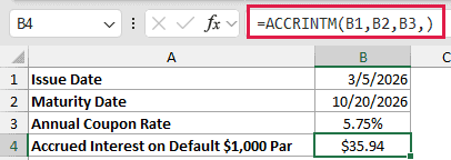
The empty fourth position makes Excel use the documented $1,000 par value. Omitting the fifth argument uses basis 0, the US 30/360 convention.

The formula returns $35.94 for a 5.75% rate from March 5 through October 20, 2026.

Pro Tip: Keep the trailing comma when you want Excel’s default par value. In native testing, removing that comma made the shortened formula fail.

Example 3: Compare Day-Count Basis Results

The basis argument controls how Excel counts or scales the days between the two dates.

Below is one security card beside the five supported basis codes and their conventions. The Accrued Interest column is ready for formulas.

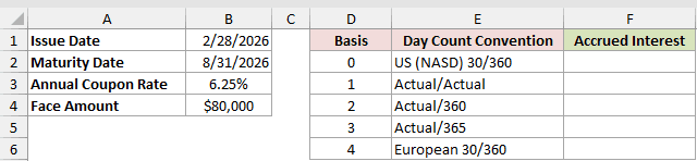
I want to calculate the same security under every day-count basis.

Enter this formula in F2, then fill it down through F6:

=ACCRINTM($B$1,$B$2,$B$3,$B$4,D2)

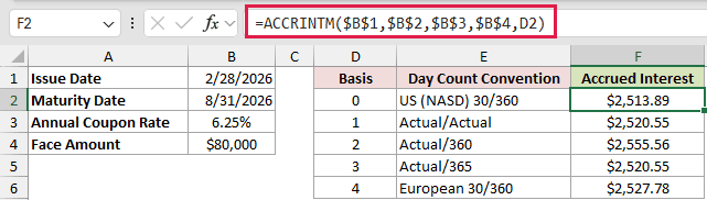
The absolute references keep the security inputs fixed. The relative D2 reference changes to the basis code on each row.

The results range from $2,513.89 under basis 0 to $2,555.56 under basis 2. Bases 1 and 3 both return $2,520.55 for these dates.

Use the basis specified in the security’s documentation. It is a contract convention, not a display preference.

Example 4: Calculate the Amount at Maturity

ACCRINTM can feed a second calculation that adds interest to the face amount.

Below is a one-year security with a $125,000 face amount and 4.8% annual coupon rate. Two result cells are ready for the calculations.

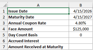
I first want to calculate the interest paid at maturity.

Here is the ACCRINTM formula:

=ACCRINTM(B1,B2,B3,B4,B5)

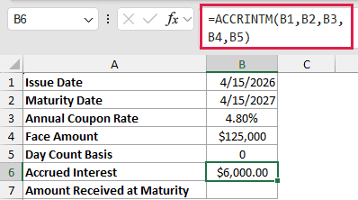
The formula returns $6,000.00. That is one full year of interest on the $125,000 face amount.

Next, add the face amount to the accrued interest:

=B4+B6

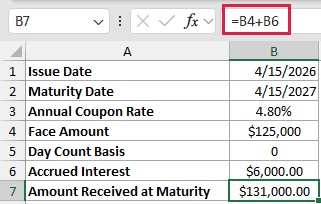
The second formula returns $131,000.00. It uses the ACCRINTM result already calculated in B6.

Tips & Common Mistakes

ACCRINTM is for securities that pay interest at maturity. Use ACCRINT for securities with periodic coupon payments.
Enter valid Excel dates or use the DATE function. Text dates can return #VALUE!.
The issue date must be earlier than the maturity date. Otherwise, Excel returns #NUM!.
The rate and par value must both be greater than zero.
Basis must be an integer from 0 through 4. Excel truncates a decimal basis to an integer.
Plain range arguments returned #VALUE! in native Excel testing. Use one scalar formula per row and fill down.

I covered scalar register calculations, Excel’s $1,000 default par value, basis comparisons, and the total amount received at maturity.

I hope you found this article helpful.