When creating sample data, you may be required to generate random names. You will find that this is a fairly routine task.
In this tutorial, I will show you how to generate random names in Microsoft Excel. Additionally, you will discover how to generate a list of five random names.
So let’s get started.
Note: In this article, we are covering the methods to generate a list of random names, and not about randomizing a list of existing names.
Generate Random Names Using TEXTJOIN, XLOOKUP, and RANDBETWEEN Functions
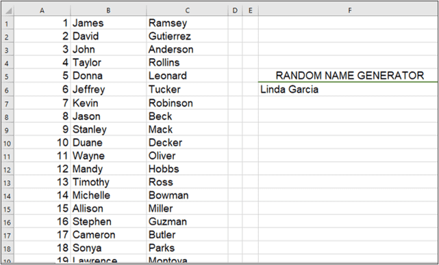
Below, we have a sample dataset showing a list of first names in column B and a list of last names in column C.
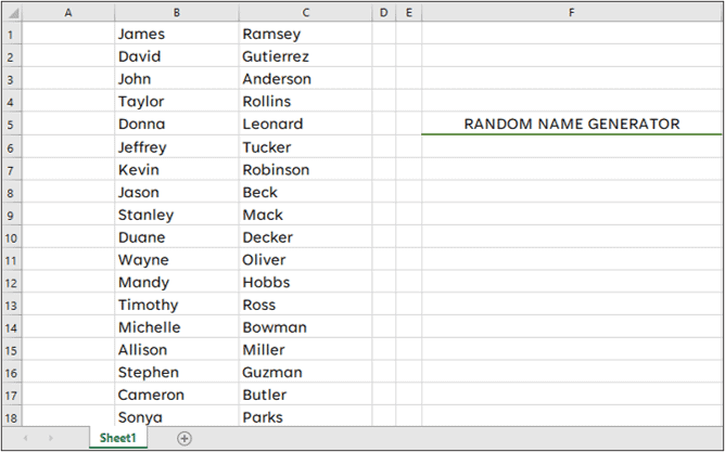
We want to create a formula in cell F6 that will generate a random full name for us using our first and last name columns.
We have 50 first names in column B and 50 last names in column C.
Creating the Helper Column
- So the first thing we are going to do is create a column with consecutive numbers. We are ultimately going to refer to this column in our formula. So in cell A1 enter the number 1, and then in cell A2, enter the number 2.
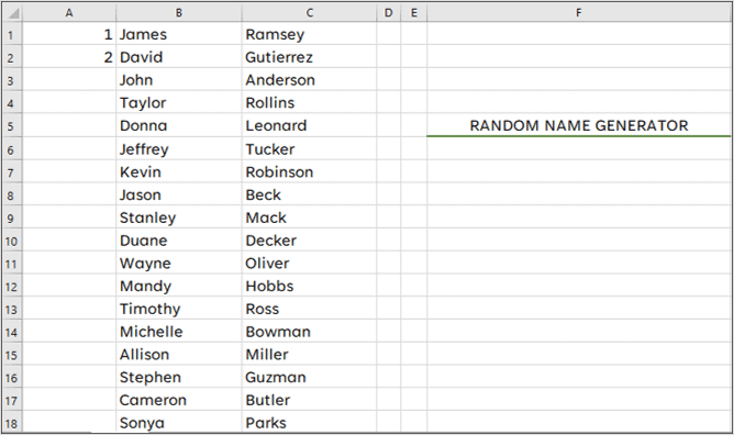
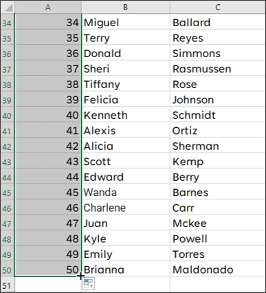
- Select range A1:A2, and using the fill handle, drag down the column to create a consecutive number series.
The next thing we need to do, since we intend to use our RANDBETWEEN Function, is to change the Calculation Options from Automatic to Manual.
The RANDBETWEEN Function is a volatile function that will recalculate every time a change is made in our workbook.
So if we don’t set the Calculation Options to Manual, we will get a new full name generated whenever we make any change to our workbook.
Change the Calculation Mode
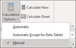
- Go to the Formulas Tab, and in the Calculation Group, select Calculation Options. Change from the default Automatic selection to Manual.

This will allow us to make changes to the workbook without the formula updating all the time because of the RANDBETWEEN Function.
Creating the Formula to Generate Random Names
In order for us to create a random full name generator in cell F6, we need to use the TEXTJOIN, XLOOKUP, and RANDBETWEEN Functions in one formula.
- So in cell F6 enter the following formula.
=TEXTJOIN(" ",TRUE,XLOOKUP(RANDBETWEEN(1,50),A1:A50,B1:B50,,0,), XLOOKUP(RANDBETWEEN(1,50),A1:A50,C1:C50,,0,))
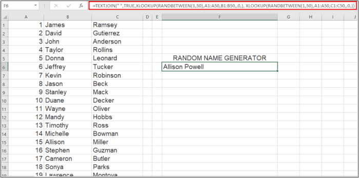
- Upon pressing Enter, the formula should generate a random full name based on a combination of first name and last name.
When you would like to generate a new random name, you can simply press F9 on the keyboard for Excel to recalculate the formula.
Formula Explanation
In a nutshell, our formula uses the TEXTJOIN Function to combine our potential two strings of text (first name and last name), which will be returned by the other functions.
The TEXTJOIN Function is used to combine text strings where one specifies a delimiter. It is only available in later versions of Office.
The syntax of the TEXTJOIN Function is as follows:
=TEXTJOIN(delimiter, ignore_empty, text1, [text2], …) where:
- delimiter denotes a text string, such as a comma or a space that will be used to separate the other text strings.
- ignore_empty tells the function whether to ignore the empty text. If this parameter is set to TRUE, the function ignores the empty cells.
- text1, text 2, … indicates the text strings the function will combine, separated by the delimiter. These text strings can be a single value or a range of cells in each case.
When honing into our formula, we see our first text string, i.e., the first name, is returned by an XLOOKUP Function.
The XLOOKUP Function is a new function available to Office 365 users. It is a more advanced version of its earlier predecessors, VLOOKUP/HLOOKUP.
It’s used to search through an array or range and return a matching item in another range or array based on the input value.
The syntax of the XLOOKUP Function is:
=XLOOKUP(lookup_value, lookup_array, return_array, [if_not_found],[match_mode], [search_mode]) where:
- lookup_value is required and is the value that we want to lookup and find a match for.
- lookup_array is the first array of interest that we want the function to search through.
- return_array is the second array of interest which Excel retrieves the matching value from.
- if_not_found is an optional parameter and allows you to specify a user-friendly text in the case where a match is not found. If this is left empty, then the #N/A error is returned.
- match_mode specifies the type of match. 0 indicates an exact match, and if no matches are found, #N/A is returned. -1 indicates an exact match or next smaller. 1 indicates an exact match or next larger. 2 allows one to perform a wildcard character match. This is an optional value, and 0 is the default.
- search_mode specifies the search mode you’d like to be used. If 1, which is the default, is specified, then the function searches from first to last. If -1 is specified, then the search is from last to first. If 2 is used, then the search is binary on ascending sorted data. If -2 is specified, then the search is binary on descending sorted data.
So in our first XLOOKUP Function, we are letting the RANDBETWEEN Function select a random number between 1 and 50 as our lookup value.
Let’s just remind ourselves that our lookup_array in column A.
In other words, we are telling the function to randomly pick a number from column A. Since our return_array is column B, the matching corresponding value is found in column B.
This first XLOOKUP Function thus returns a random first name from Column B.
Our second XLOOKUP Function follows a similar logic to that of the first one. However, this time we want to select a matching last name from column C. Our return_array, in this case, is column C.
The first name and the last name are combined through our TEXTJOIN Function, with a space specified as the delimiter between them.
Every time, we want to generate a new random full name, we simply press F9 on the keyboard.
Note: This is the shortcut key for the Calculate Now feature.
Also read: How to Generate Random Letters in Excel?
Generate a Random List of Names Using XLOOKUP, RANDARRAY, and the CONCATENATION Operator
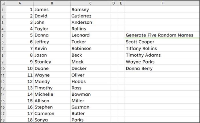
We have already seen how to generate a random full name in our example above. In this example, we want to create a list of five random full names.
We have the same sample dataset we used above, showing the Helper Column, i.e., column A, a list of first names in column B and a list of last names in column C.
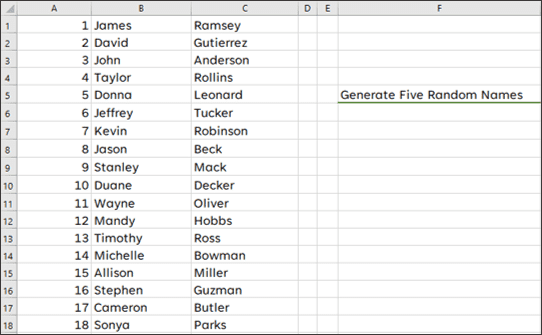
The first thing we need to do, since we intend to use our RANDARRAY function, is to change the Calculation Options from Automatic to Manual.
The RANDARRAY Function, like the RANDBETWEEN function, is a volatile function that will recalculate every time a change is made in our workbook.
Change the Calculation Mode
- Go to the Formulas Tab, and in the Calculation Group, select Calculation Options. Change from the default Automatic selection to Manual.
Creating the Formula
In order for us to create a list of five random full names, we need to use the XLOOKUP Functions, RANDARRAY Functions, and CONCATENATION operator in a formula.
- So in cell F6 enter the following formula.
=XLOOKUP(RANDARRAY(5,1,1,50,TRUE),A1:A50,B1:B50,,0) & " " &XLOOKUP(RANDARRAY(5,1,1,50,TRUE),A1:A50,C1:C50,,0)
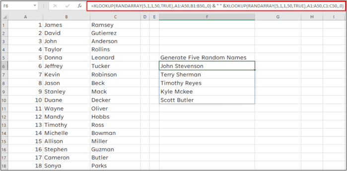
- Upon pressing Enter, we will get a spill range containing our five randomly generated full names.
If you would like to generate a list of five new full names, press F9 on your keyboard so Excel can recalculate the formula.
Formula Explanation
In this formula, we are taking full advantage of dynamic array functionality.
Dynamic array functions allow you to work with multiple input values and also return multiple values into different cells.
These functions are only available to Office 365 users. In our formula, we are utilizing the XLOOKUP and RANDARRAY dynamic array functions.
The RANDARRAY Function returns an array of numbers, within an interval that is specified.
The syntax of the RANDARRAY Function is as follows:
=RANDARRAY([rows],[columns],[min],[max],[whole_number]) where:
- rows argument is optional and indicates how many rows to fill. The default value is 1.
- columns argument is optional and indicates how many columns to fill. The default value is 1.
- min indicates the smallest value that can possibly be returned. This is optional, and if omitted, 0 is used.
- max indicates the largest value that can possibly be returned. This is optional, and if omitted, 1 is used.
- whole_number tells the function whether to return integers or decimal numbers. If TRUE integers are returned. If FALSE, then decimal numbers are returned. The default is FALSE.
The RANDARRAY Function will randomly choose and output five values, between 1 and 50.
We specified five rows, so we will get five values spilled down five rows ultimately.
Additionally, remember we have 50 first names in total, which is why our min and max parameters are 1 and 50, respectively.
In our formula, our RANDARRAY Function is basically generating our lookup values for our XLOOKUP function.
So our first XLOOKUP function is taking in a range of five random numbers between 1 and 50 as the first input.
Since it is a dynamic array function, it can use multiple values as lookup values.
These values are then found in column A, and the matching values from column B are returned in the spill range. So our first XLOOKUP Function will return five random first names.
Note: If we specified 20 rows instead of 5, then we would get 20 first names returned.
We are then using the concatenation operator to join each of our first names and last names, with a space in between them.
The second XLOOKUP Function follows the same logic as the first one, except, in this case, our matching return values are sourced from column C. This is the column that contains the last names.
We put everything together to generate five random full names, and every time we press F9, a new set is generated.
And there you have it. It’s that easy.
Also read: How to Add Comma Between Names in Excel
Generate Random Names Using Third Party Tools/Websites
Finally, you can also generate a list of random names using a third-party website such as Fake Name Generator or a tool such as ChatGPT.
Note that the names you get from these third-party tools are going to be random, and the data is not taken from any database or list of actual people’s names.
In this article, I went through three simple ways to generate random names in Excel.
I hope you found this tutorial useful, and please feel free to comment below and share your thoughts.
Other Excel articles you may also like:
- How to Generate Random Numbers in Excel (Without Duplicates)
- Get Unique Values from a Column in Excel
- How to Create Custom Lists in Excel?
- Switch First and Last Name with Comma in Excel (Reverse Names)
- How to Separate Names in Excel
- Remove Middle Name from Full Name in Excel
- How to Merge First and Last Name in Excel
- Generate All Possible Combinations from Two Lists
- Generate Random Dates in Excel
