
What price gives you a 30% margin after fees? How many production batches cover an order? How much customer churn can you afford?
Goal Seek in Excel answers these questions by working backward from a formula result to the input that produces it.
I’ll walk through seven examples, starting with pricing and moving into demand forecasts and project cash flows. Each one includes the setup, Goal Seek settings, and a checked answer.
How Goal Seek Works in Excel
Goal Seek changes one input cell until a dependent formula gets close to a number you specify.
You need three things:
- Set cell: The cell containing the formula you want to control.
- To value: The target number. For a percentage such as 30%, enter
0.3. - By changing cell: A numeric input that feeds that formula, directly or through other formulas.
The changing cell must contain a value, not a formula. Keep the other assumptions fixed while Excel searches.
The examples below use desktop Excel for Windows. Open the downloaded workbook and work in columns A:B; columns D:E contain checked solutions for comparison.
The formulas are already filled in. You can also recreate each model from the screenshots and formulas below.
Example 1: Find a Selling Price for a Target Profit Margin
Suppose you sell a product that costs $24 to make and $6 to fulfill. A marketplace takes 10% of the selling price.
You want a 30% profit margin after these costs. What should you charge?
Open the Price and Margin sheet. The starting price in B2 is $45.
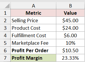
B6 calculates profit per order with =B2*(1-B5)-B3-B4. It subtracts the marketplace fee, product cost, and fulfillment cost from the selling price.
B7 divides that profit by the selling price:
=B6/B2
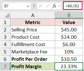
This is a margin calculation. Dividing profit by cost would give you a markup instead.
- Select B7, the profit margin formula.
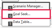
- Go to Data > What-If Analysis > Goal Seek.
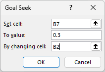
- Enter B7 in Set cell, 0.3 in To value, and B2 in By changing cell.
- Click OK to run Goal Seek. Excel displays a status dialog when it finishes.
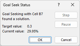
- Click OK again to keep the result, or Cancel to restore the original input.
Check the result before using it. In my test, Excel reported a solution at about $49.96, leaving the margin slightly below 30%.
That happens because Goal Seek uses a tolerance. Its “solution found” message doesn’t promise an exact match.
For this model, enter 50 in B2 and check B7 again. The price gives $15 profit per order and exactly 30% margin.
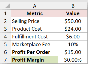
You can verify the price independently: $30 of costs divided by (1 - 10% - 30%) equals $50.
The Solution panel uses this checked price. It excludes any costs you haven’t included, such as returns or general overhead.
Example 2: Find the Conversion Rate an Advertising Campaign Needs
Suppose a campaign brings 12,000 visits to your website. Each order earns $80 in revenue and costs $50 to supply.
Advertising costs $3,600. You want $2,400 profit after advertising and variable order costs.
Open Campaign Conversion. B3 starts at a 1% conversion rate.
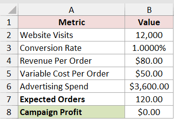
B7 uses =B2*B3 to calculate expected orders. At 1%, that’s 120 orders.
The profit formula in B8 is:
=B7*(B4-B5)-B6
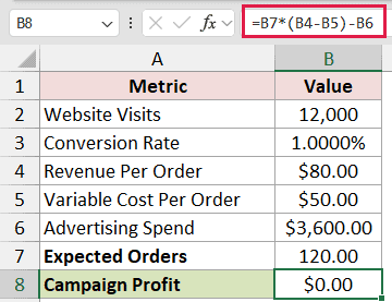
At the starting conversion rate, the campaign only covers its costs. Use Goal Seek to find the rate required for the profit target.
- Select B8 and open Data > What-If Analysis > Goal Seek.
- Set B8 to 2400 by changing B3.
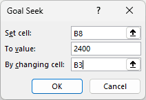
- Click OK, then accept the result in the status dialog.
Excel finds a conversion rate of about 1.6667%. That means 200 orders, each contributing $30 before advertising costs.
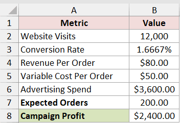
The check is straightforward: 200 orders × $30 contribution, minus $3,600 advertising, leaves $2,400.
Goal Seek can follow a chain of formulas. B8 doesn’t refer directly to B3, but B7 links them.
This is a planning threshold, not a prediction that the campaign will achieve that rate. Visitor count, order value, and costs remain fixed in this model.
Example 3: Calculate Production Batches After Rejects
Suppose each production batch makes 80 units, and you expect 5% to be rejected. You need at least 1,000 usable units.
Open Production Batches. B2 starts at 10 batches, producing 760 usable units under the assumed reject rate.
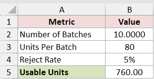
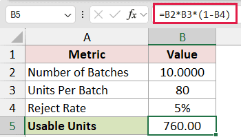
B5 calculates usable output:
=B2*B3*(1-B4)
- Select B5 and open Goal Seek.
- Set B5 to 1000 by changing B2.
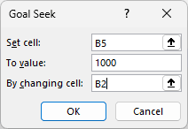
- Run Goal Seek and keep the result.
Excel returns approximately 13.1579 batches.
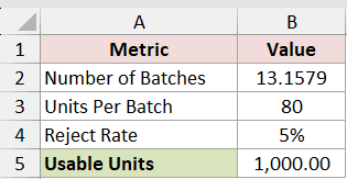
That solves the equation, but you can’t schedule part of a batch in this scenario. Round the answer up to 14 batches.
Enter 14 in B2. B5 becomes 1,064 usable units.
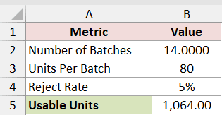
Thirteen batches would produce only 988 usable units. Fourteen is therefore the smallest whole-batch plan that meets the target under these assumptions.
The workbook’s Practical Check calculates this rounded answer separately. Actual rejects can vary, so 1,064 is a modeled quantity, not a production guarantee.
Keep rounding outside the formula Goal Seek is solving. A rounded output changes in jumps and can make it harder for Excel to find a solution.
Example 4: Find the Maximum Monthly Churn Rate
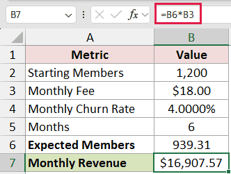
Suppose a membership business has 1,200 members paying $18 a month. You want monthly revenue of at least $18,000 after six months.
Assume no new members join and the same percentage leaves each month. How low does monthly churn need to be?
Open Membership Churn. The starting monthly churn rate in B4 is 4%.
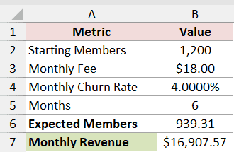
B6 calculates retained members with =B2*(1-B4)^B5. The exponent applies six monthly retention periods.
B7 converts retained members into monthly revenue:
=B6*B3
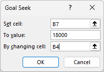
- Select B7 and open Goal Seek.
- Set B7 to 18000 by changing B4.
- Run Goal Seek and accept the result.
The threshold is approximately 2.992988% monthly churn, displayed as 2.9930% in the workbook.
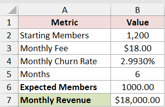
At the unrounded threshold, about 1,000 members remain, producing $18,000 in monthly revenue. This is the revenue level after six months, not total revenue over those months.
For a practical target stated to two decimal places, aim for 2.99% or lower. Rounding up to 3.00% would put revenue slightly below the target.
The direction matters here: lower churn produces more retained revenue. Goal Seek finds the boundary; you decide which side meets your requirement.
Example 5: Work Backward From a Mileage Budget
Suppose a van rental costs $210 and includes 500 miles. Extra mileage costs $0.28 per mile, while fuel costs an estimated $0.12 per mile.
Your total budget is $400. How far can you drive?
Open Mileage Budget. The starting trip distance is 400 miles.
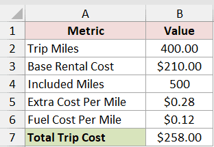
B7 calculates the total cost:
=B3+MAX(0,B2-B4)*B5+B2*B6
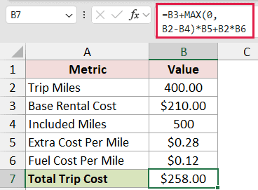
MAX(0,B2-B4) charges only for miles beyond the included allowance. Fuel applies to every mile.
- Select B7 and open Goal Seek.
- Set B7 to 400 by changing B2.
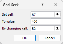
- Run Goal Seek and keep the result.
Excel finds 825 miles.
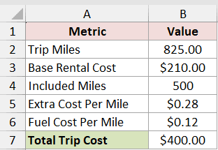
The cost breaks down as follows:
- Base rental: $210.
- Extra mileage: 325 × $0.28 = $91.
- Fuel: 825 × $0.12 = $99.
- Total: $400.
This formula changes its rate of increase after 500 miles, but the total cost remains continuous. Goal Seek can work across that change.
Use nonnegative distances when interpreting the result. Goal Seek doesn’t know a negative trip distance is impossible, and it doesn’t enforce a minimum or maximum input.
Example 6: Find Two Prices That Reach the Same Profit
A higher price doesn’t always mean more profit. If demand falls as the price rises, the same profit target can have two answers.
Suppose a desk-lamp seller uses this simplified demand model: expected units sold equal 1,000 minus 10 times the selling price.
Each lamp costs $20 to supply, and fixed costs are $6,000. The profit target is $6,000.
Open Price and Demand. The starting selling price in B2 is $35.
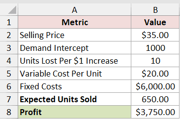
B7 calculates expected demand with =B3-B4*B2. B8 calculates profit:
=(B2-B5)*B7-B6
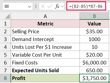
This is an assumed relationship for practicing Goal Seek. A real pricing decision needs a demand estimate supported by your own data.
- Select B8 and open Goal Seek.
- Set B8 to 6000 by changing B2.
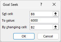
- Run Goal Seek from the starting price of $35 and accept the result.
Excel finds a price of approximately $40, with expected sales of 600 lamps.
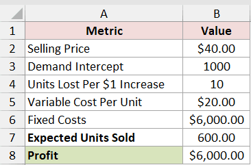
Now enter 85 in B2 and run Goal Seek again with the same target and settings.
This time, Excel finds approximately $80, with expected sales of 200 lamps.
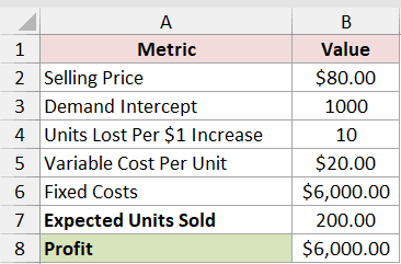
Both answers produce $6,000 profit:
- At $40:
($40 - $20) × 600 - $6,000 = $6,000. - At $80:
($80 - $20) × 200 - $6,000 = $6,000.
The starting value can affect which answer Goal Seek finds. It doesn’t list every solution or tell you which price is preferable.
It also doesn’t maximize profit. In this model, a $60 price produces $10,000 profit, which is higher than the target we asked it to reach.
Use Solver when your question is “Which price gives the highest profit?” or when price and demand need explicit constraints.
Example 7: Find the Cash Flow Growth Needed for a Project
Suppose a project requires $80,000 today and is expected to generate $18,000 at the end of year one.
You use a 10% annual discount rate and evaluate five years of cash flows. What annual cash flow growth would bring net present value to zero?
Open Project Growth. B4 starts at 5% growth.
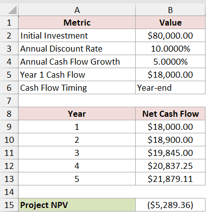
The worksheet builds the forecast first:
- B9:
=$B$5, the year-one cash flow. - B10:
=B9*(1+$B$4), the year-two cash flow. - B11:B13: The same growth calculation copied down for years three through five.
B15 calculates the project’s net present value:
=NPV(B3,B9:B13)-B2
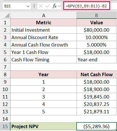
The $80,000 investment happens today, so it sits outside NPV. The five cash flows inside NPV occur at the ends of equally spaced annual periods.
- Select B15 and open Goal Seek.
- Set B15 to 0 by changing B4.
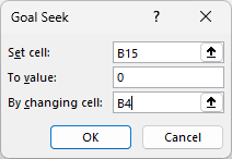
- Run Goal Seek and accept the result.
Excel finds annual cash flow growth of approximately 8.763967%, displayed as 8.7640%.
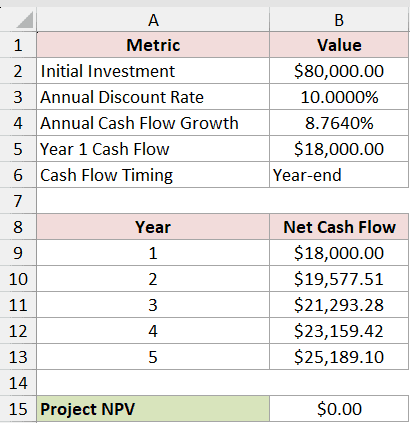
At that rate, the five future cash flows have a present value of about $80,000. Subtracting the initial investment leaves an NPV near zero.
The discount rate stays at 10%. We’re solving for growth in cash flows, not for the discount rate that would make NPV zero.
This model assumes constant growth, year-end cash flows, and no terminal value after year five. Add any relevant taxes or other costs to your own forecast.
Goal Seek Settings for All Seven Examples
Use these settings in the starting model in columns A:B of each workbook sheet.
| Example | Set cell | To value | By changing cell | Checked answer |
|---|---|---|---|---|
| Selling price and margin | B7 | 0.3 | B2 | $50 price for exactly 30% margin |
| Campaign conversion | B8 | 2400 | B3 | About 1.6667% |
| Production batches | B5 | 1000 | B2 | About 13.1579; use 14 whole batches |
| Membership churn | B7 | 18000 | B4 | About 2.992988%; aim for 2.99% or lower |
| Mileage budget | B7 | 400 | B2 | 825 miles |
| Price and demand | B8 | 6000 | B2 | $40 or $80, depending on starting value |
| Project cash flow growth | B15 | 0 | B4 | About 8.7640% |
Why Goal Seek Sometimes Gives an Unexpected Answer
The result is close, but not exact. Goal Seek uses numerical iteration and a tolerance. Check the formula result before using the changed input.
The pricing example demonstrates this: a displayed solution near $50 can still leave margin below 30%. More decimal places reveal the difference; formatting doesn’t change the underlying value.
The changing cell isn’t connected to the formula. Change that input manually and check whether the Set cell responds. If it doesn’t, inspect the formula references.
The Set cell contains a fixed number. Replace it with the formula you want Excel to solve. The changing cell, meanwhile, should contain an editable numeric value.
The target isn’t feasible. In the mileage model, even a zero-mile trip costs $210. A $200 budget has no solution with nonnegative miles.
The model has more than one solution. Try another sensible starting input, as shown in the price-and-demand example. One successful run doesn’t prove uniqueness.
The model rounds or jumps between outputs. Functions that round intermediate results can prevent the formula from ever reaching the exact target.
The answer violates a business rule. Goal Seek may return a fraction of a batch, an unsuitable percentage, or an input outside your allowed range.
For whole numbers, bounds, multiple changing cells, or optimization, Solver supports constraints that Goal Seek doesn’t offer.
Common Questions About Goal Seek
Where is Goal Seek in Excel?
In desktop Excel for Windows, go to Data > What-If Analysis > Goal Seek. You can also press Alt, A, W, G in sequence on the English Windows ribbon.
Can Goal Seek change more than one cell?
No. It changes one input per run. Use Solver when you need Excel to adjust several inputs together.
Does Goal Seek update automatically when my assumptions change?
No. The formulas recalculate, but the solved input remains a value. Run Goal Seek again after changing assumptions such as costs, fees, or traffic.
Can I use a target stored in another cell?
The To value box expects a number. If your target is stored elsewhere, use a formula that subtracts the target from the calculated result, then seek zero.
Is Goal Seek available in Excel for the web?
These instructions use the built-in desktop feature. Open the workbook in desktop Excel to follow the Goal Seek steps shown here.
How do I undo Goal Seek?
Click Cancel in its status dialog to restore the starting input. After accepting the result, use Ctrl+Z immediately to undo the change.
For the built-in feature’s setup requirements, see Microsoft’s Goal Seek guide.
I use Goal Seek when the desired result is clear and there’s one input to find. The part I always check afterward is whether the answer works outside the equation.
Other Excel articles you may also like:
