How to Do Sensitivity Analysis in Excel

If you want to see how changes in price or sales volume affect profit, replacing one input at a time gets tedious. It also makes it easy to lose track of the values you have tested.

Excel has four useful What-If Analysis tools for this job. In this article, I will use the same monthly profit model to show you how each one works.

Which Sensitivity Analysis Method Should You Use?

The right method depends on the question you are trying to answer.

Method	Use It When You Want To
One-variable Data Table	Test several values for one input
Two-variable Data Table	Test combinations of two inputs
Goal Seek	Find the input needed to reach a target result
Scenario Manager	Save and compare named sets of inputs

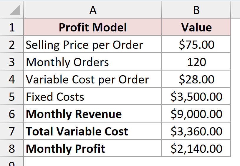
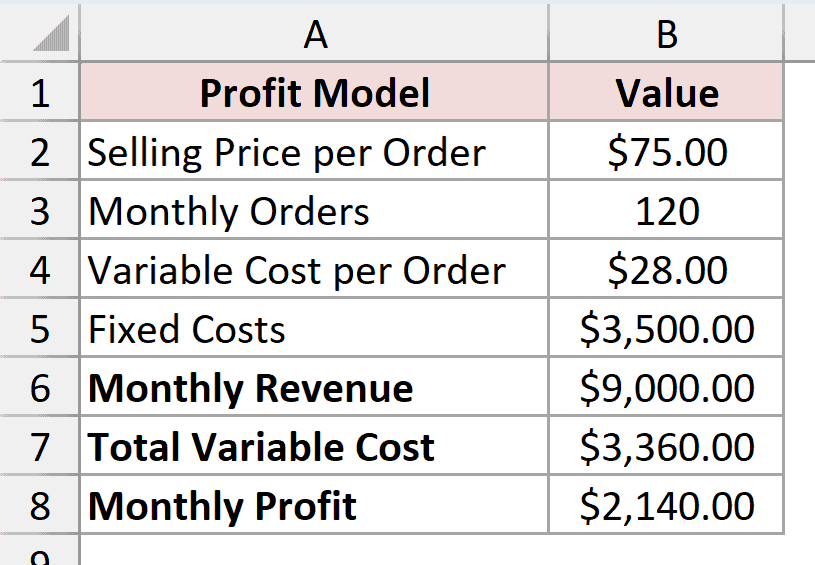
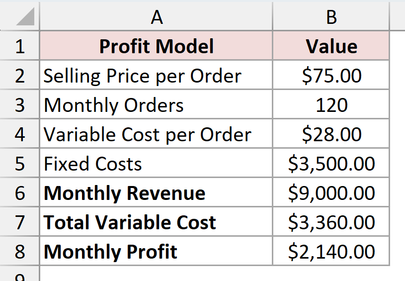
The workbook uses a small cafe profit model. The selling price is $75 per order, monthly orders are 120, variable cost is $28 per order, and fixed costs are $3,500.

Monthly profit is calculated as selling price minus variable cost, multiplied by monthly orders, less fixed costs. With the starting values, the profit is $2,140.

Method #1: Using a One-Variable Data Table

A one-variable Data Table shows how one formula result changes when you substitute several values into one input cell. I use this when I want a complete list of results instead of testing the input manually.

In the first worksheet, Monthly Orders is in B3 and Monthly Profit is in B8. I want to test order volumes from 80 to 180 while leaving the other inputs unchanged.

Here are the steps to create the one-variable Data Table:

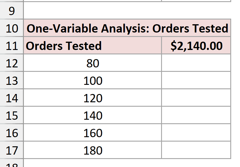
1. Enter the order volumes you want to test in A12:A17. In this example, the values are 80, 100, 120, 140, 160, and 180.

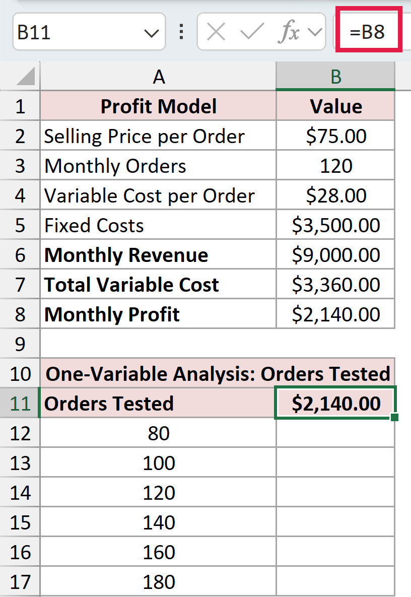
2. In B11, enter a reference to the result you want Excel to calculate for each order volume.

=B8

3. Select A11:B17, including the result reference, the order volumes, and the empty result cells.

4. On the Data tab, click What-If Analysis and choose Data Table.
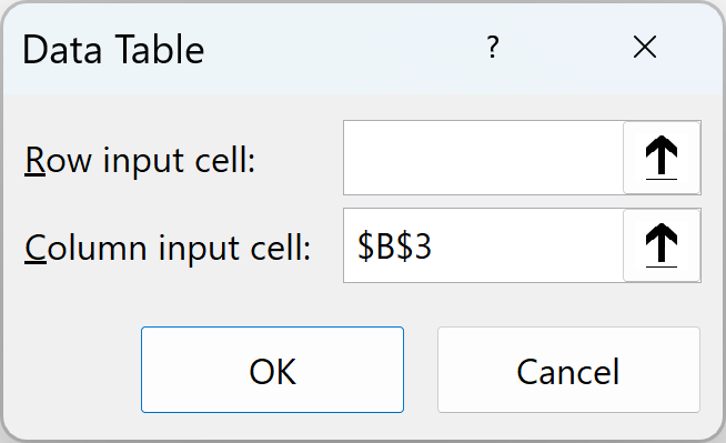
5. Leave Row input cell empty. Set Column input cell to $B$3, then click OK.

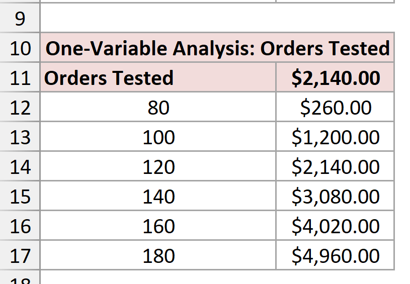
Excel returns monthly profits of $260, $1,200, $2,140, $3,080, $4,020, and $4,960. Each additional 20 orders adds $940 in monthly profit.

Note: The test values run down a column, so B3 belongs in the Column input cell box. If the values ran across a row, you would use the Row input cell box instead.

Method #2: Using a Two-Variable Data Table

If two inputs may change together, a two-variable Data Table is more useful. It calculates one result formula for every combination in a row-and-column grid.

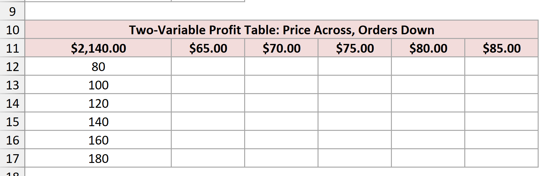
This worksheet tests Selling Price per Order in B2 and Monthly Orders in B3. Prices run from $65 to $85, while order volumes run from 80 to 180.

Here are the steps to create the two-variable Data Table:

1. Enter the selling prices across B11:F11 and the monthly order volumes down A12:A17.

2. In A11, enter a reference to Monthly Profit.

=B8

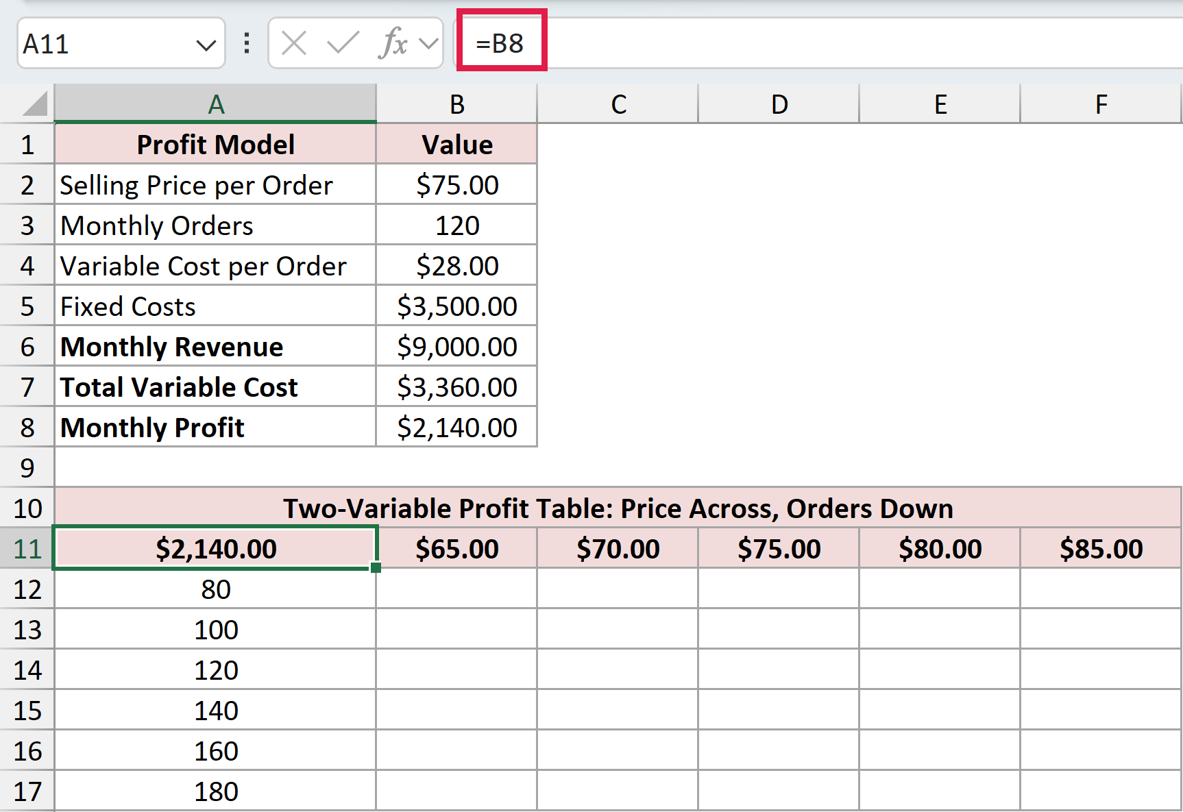
3. Select the entire table area, A11:F17.

4. On the Data tab, click What-If Analysis and choose Data Table.
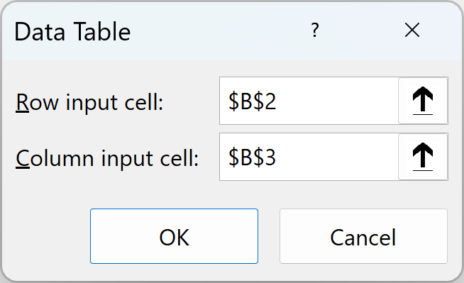
5. Set Row input cell to $B$2 because prices run across the top. Set Column input cell to $B$3 because order volumes run down the side, then click OK.

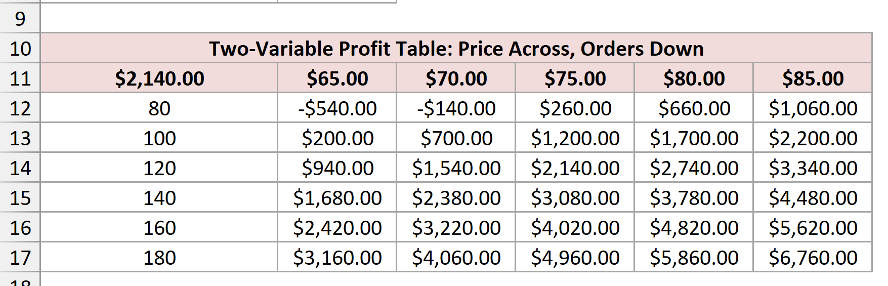
At the original price of $75 and 120 monthly orders, the table returns the starting monthly profit of $2,140. At $85 and 180 orders, monthly profit increases to $6,760.

The grid also shows the combinations that lose money. For example, 80 monthly orders at $65 per order produce a $540 loss.

Note: A two-variable Data Table can evaluate only one result formula. If you need to compare several result formulas, create separate tables or use a one-variable table with multiple result columns.

Method #3: Using Goal Seek

Goal Seek works backward. You give Excel the formula result you want, and it changes one input value until the formula reaches that target.

In this example, I want Monthly Profit in B8 to equal $3,000. Excel will change the Selling Price per Order in B2 while monthly orders and costs stay fixed.

Here are the steps to run Goal Seek:

1. On the Data tab, click What-If Analysis and choose Goal Seek.
2. Set the Set cell box to $B$8.
3. Enter 3000 in the To value box.
4. Set the By changing cell box to $B$2, then click OK.

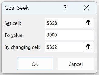
Goal Seek finds a selling price of $82.1666667, which displays as $82.17 with currency formatting. After you accept the solution, B8 shows the target monthly profit of $3,000.

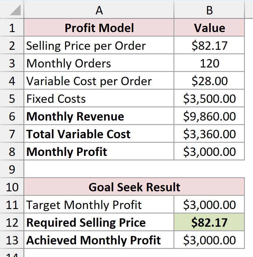
The workbook repeats the required selling price in B12 and the achieved monthly profit in B13. That makes the result easy to find when you open the completed file later.

Note: The Set cell must contain a formula, and that formula must depend on the changing cell. Goal Seek changes only one input and does not apply constraints.

Method #4: Using Scenario Manager

Scenario Manager is useful when you have a few complete cases to compare. Each scenario stores a named set of input values, so you can switch between them or create a summary report.

This example changes Selling Price per Order in B2 and Monthly Orders in B3. Monthly Profit in B8 is the result cell.

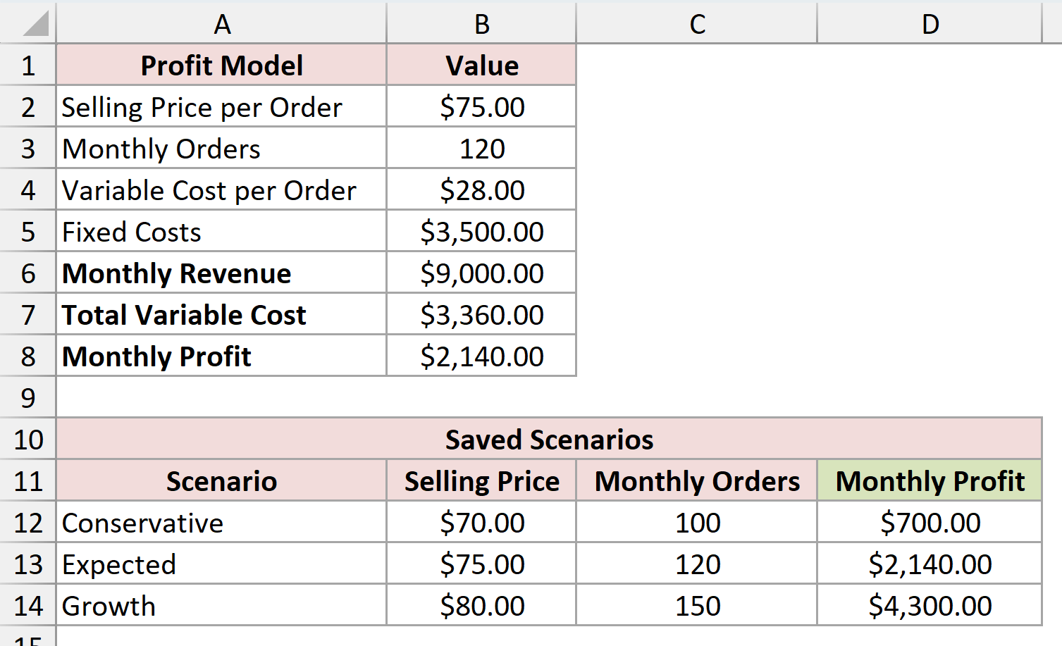
The workbook uses these three scenarios:

Scenario	Selling Price	Monthly Orders	Monthly Profit
Conservative	$70	100	$700
Expected	$75	120	$2,140
Growth	$80	150	$4,300

Here are the steps to create the scenarios:

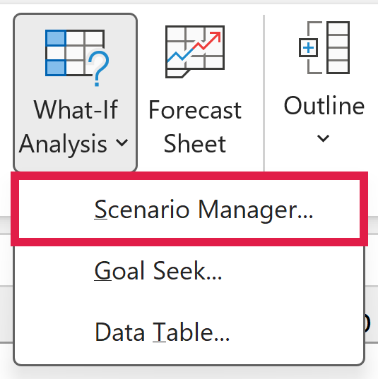
1. On the Data tab, click What-If Analysis, choose Scenario Manager, and click Add.

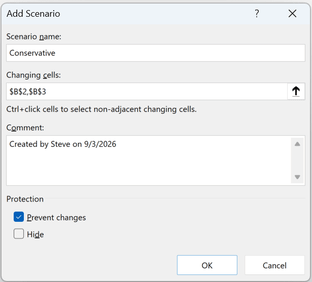
2. Enter Conservative as the scenario name. Set Changing cells to $B$2,$B$3, then click OK.

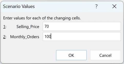
3. Enter 70 for Selling Price and 100 for Monthly Orders. Click Add and repeat the process for Expected and Growth.

4. In the Scenario Manager, select a scenario and click Show to place its saved values into B2 and B3.
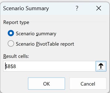
5. To compare all three scenarios, click Summary. Choose Scenario summary, set Result cells to $B$8, and click OK.

Excel creates a new Scenario Summary worksheet with the current values and all three saved scenarios. Because the workbook uses named cells, the report shows Selling Price, Monthly Orders, and Monthly Profit instead of cell references.

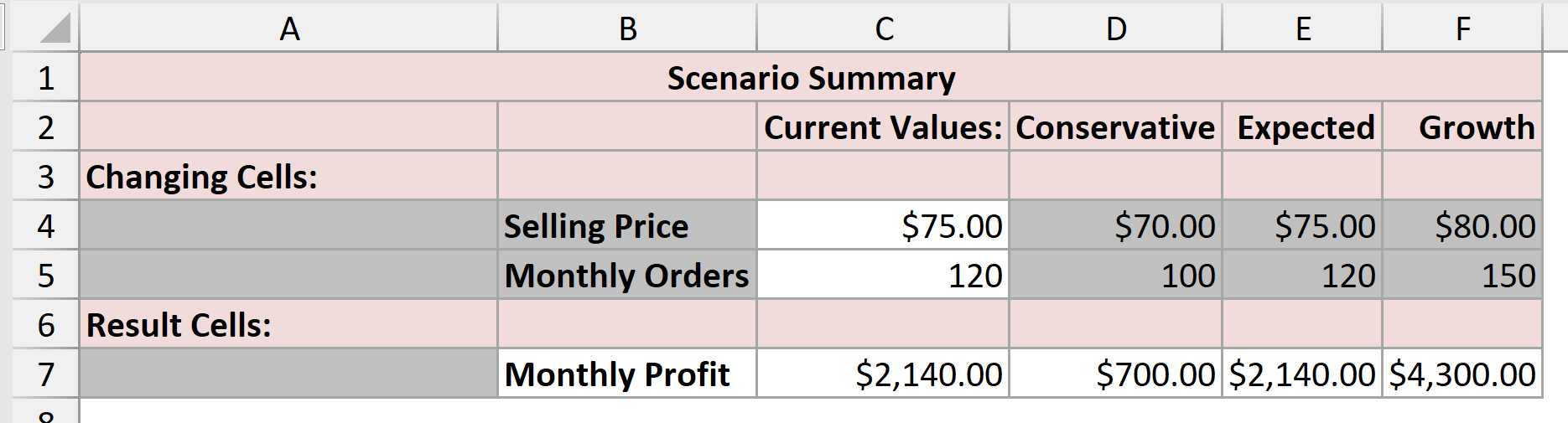
Note: Scenario Summary reports do not update automatically. If you change a saved scenario, create a new summary report to see the revised values.

Additional Notes About Sensitivity Analysis in Excel

• Data Tables recalculate with the workbook when calculation is set to Automatic. If you use Automatic Except for Data Tables, select the table formulas and press F9 when you want to refresh them.
• You cannot edit one result inside a Data Table. Excel treats the output as one table calculation, so you must select and clear the entire result range if you want to remove it.
• Goal Seek handles one changing input. Use Solver when you need several changing cells, limits, or an optimal solution.
• Scenario Manager allows up to 32 changing cells in each scenario, and you can create as many named scenarios as you need.

Frequently Asked Questions

Why does a Data Table show the same result in every cell?

Check that the result formula depends on the row or column input cell you selected. Also check the workbook’s calculation setting, since a table can show old results when Data Table calculation is disabled.

What does {=TABLE(,B3)} mean in Excel?

Excel creates this special formula for a column-oriented Data Table. The empty first argument means there is no Row input cell, while B3 is the Column input cell. Excel adds the curly brackets automatically.

Is sensitivity analysis the same as What-If Analysis?

Sensitivity analysis is one use of Excel’s What-If Analysis tools. Data Tables are the most direct sensitivity tool, while Goal Seek and Scenario Manager answer related questions about targets and saved cases.

Can a Data Table test more than two inputs?

No. A Data Table supports one or two input cells. Use Scenario Manager for selected combinations or Solver when several inputs and constraints must be handled together.

Conclusion

I use Data Tables when I want to see a range of possible outcomes, Goal Seek when I have a target, and Scenario Manager when I want to save specific cases.

I hope you found this article helpful.

Other Excel articles you may also like:

• How to Run a Monte Carlo Simulation in Excel
• How to Calculate IRR With Excel