
Margin formulas in Excel help you price products and check how much of each sale you keep after costs.
Margin and markup both measure profit, but you divide by different amounts.
With margin, you divide by the selling price; with markup, you divide by the cost, so one item gives you two very different percentages.
I’ll show you how to calculate those percentages and set a selling price from the margin you want.
Profit Margin vs Markup
Both start with profit, which is the selling price minus the cost. You then divide that profit by either the price or the cost.
- Profit Margin = (Selling Price – Cost) / Selling Price
- Markup = (Selling Price – Cost) / Cost
For a Ceramic Mug costing $4.50 and selling for $12.00, you keep $7.50 before other expenses.
You get a 62.5% margin by dividing $7.50 by $12.00. You get a 166.7% markup by dividing the same $7.50 by $4.50.
Your margin stays below 100%. Businesses usually report margin, while you’ll often use markup when setting prices from cost.
How to Calculate Profit Margin in Excel
Let me put that price-based calculation into Excel so you can check each product’s gross profit margin.
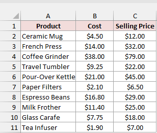
Below I have a dataset of products, with cost in column B and selling price in column C.
I want the profit margin for each product in column D.
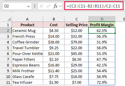
Enter this formula in D2. In Excel 365 or 2021, it spills down the column automatically.
=(C2:C11-B2:B11)/C2:C11
How does this formula work?
You subtract each product’s cost from its selling price with C2:C11-B2:B11. Then you divide by C2:C11 to measure profit as a share of the price.
For the Ceramic Mug, you subtract $4.50 from $12.00 to get $7.50. You then divide $7.50 by $12.00, giving you a 62.5% margin.
You’ll initially see decimals such as 0.625. Format column D with Percent Style on the Home tab, or press Ctrl+Shift+%.
You’ll find Percent Style in the Number group. It shows no decimal places, so click Increase Decimal once to match the one-decimal percentages shown above.
In older Excel versions, you can enter this single-cell formula in D2 and copy it down.
=(C2-B2)/C2
Note: You’ll get #DIV/0! when a product’s selling price is 0. Use =IF(C2:C11=0,"",(C2:C11-B2:B11)/C2:C11) to leave that row’s result blank instead.
How to Calculate Markup in Excel
Now you can compare that same profit with the product’s cost instead of its selling price.
Below I have a dataset of products, with cost in column B and selling price in column C. I want the markup percentage in column D.
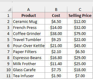
Type this formula in D2 to have the results spill down the column.
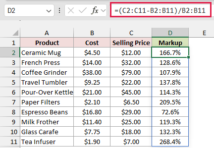
=(C2:C11-B2:B11)/B2:B11
How does this formula work?
You still subtract cost from selling price to find profit. But you divide by B2:B11, the cost, instead of the selling price.
For the Ceramic Mug, you divide $7.50 profit by $4.50 cost, giving you a 166.7% markup.
Your margin stays below 100%. Markups can go higher, such as the Tea Infuser’s 268.4%.
You can also use =C2:C11/B2:B11-1 for the same answer.
In older Excel versions, you can enter this single-cell formula in D2 and copy it down.
=(C2-B2)/B2
How to Calculate Selling Price From a Target Margin
Once you know the margin you want, you can work backward to a selling price.
Below I have products with cost in column B and target margin in column C. I want the selling price for each product in column D.
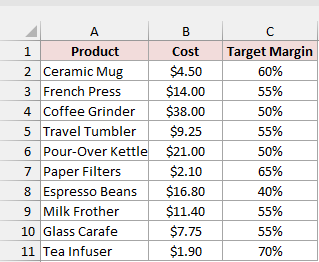
Enter the formula in D2. The selling prices spill down the column automatically.
=B2:B11/(1-C2:C11)
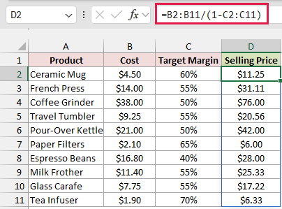
How does this formula work?
If you want to keep 50% of the selling price as profit, your cost must make up the other 50%.
You use 1-C2:C11 to find that cost share, then divide the cost by it to find the selling price.
For the Coffee Grinder, you divide $38.00 by 0.5 to get $76.00. Your $38.00 profit is then 50% of the $76.00 selling price.
Don’t use Cost*(1+Margin) for a target margin. You’d price the Coffee Grinder at $57.00, which gives you only a 33.3% margin.
In older Excel versions, you can enter this single-cell formula in D2 and copy it down.
=B2/(1-C2)
Note: You’ll get #DIV/0! with a target margin of 100%, and a negative price with anything above 100%. Your target margin must always stay below 100%.
How to Calculate Selling Price From a Markup
If you’re pricing from a markup instead, you need to multiply your cost rather than divide by a margin share.
Below I have products with cost in column B and markup in column C. I want the selling price in column D.
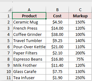
Start in D2 with this formula, which spills the selling prices down the column.
=B2:B11*(1+C2:C11)
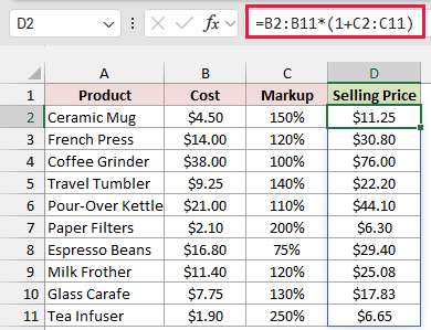
How does this formula work?
You add 1 to the markup to include the original cost in your selling price. With a 150% markup, you multiply the cost by 2.5.
For the Ceramic Mug, you multiply $4.50 by 2.5 to get $11.25.
You get $11.25 in the target-margin example too, because a 150% markup and a 60% margin give you the same selling price.
In older Excel versions, you can enter this single-cell formula in D2 and copy it down.
=B2*(1+C2)
How to Convert Margin to Markup (and Back)
You might get a supplier’s price sheet with markups while your reports use margins. I use these conversions to compare the percentages on the same basis.
Below I have margin percentages in column A. I want the matching markup percentages in column B.
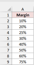
Enter this in B2 and the matching markups spill down the column.
=A2:A9/(1-A2:A9)
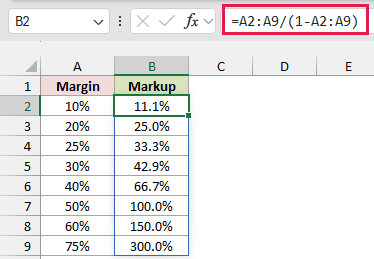
You get a 100% markup from a 50% margin, and a 150% markup from a 60% margin.
For the reverse calculation, I have markup percentages in column A on another sheet. I want the matching margins in column B.
Use this formula in B2. It spills the margin results down the column.
=A2:A9/(1+A2:A9)
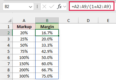
You get a 50% margin from a 100% markup, and a 75% margin from a 300% markup.
How do these formulas work?
With margin, you measure profit against the price, so 1-margin is the cost’s share of that price. You divide the margin by that share to get markup.
With markup, you measure profit against cost, so 1+markup expresses the price relative to cost. You divide the markup by that amount to get margin.
How to Calculate Gross and Net Profit Margin
Gross profit margin subtracts only the cost of goods sold from revenue, the money you earn from sales.
Net profit margin also subtracts operating expenses such as rent, wages, and marketing. It shows what’s really left from each dollar of sales.
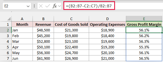
Below I have a monthly profit and loss summary. You can see revenue in B, cost of goods sold in C, and operating expenses in D.
I want the gross profit margin in column E and net profit margin in column F.
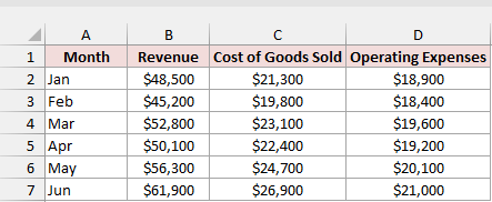
Enter this gross profit margin formula in E2. The results spill down the column.
=(B2:B7-C2:C7)/B2:B7
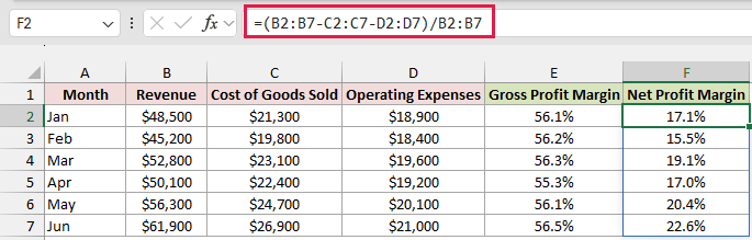
For net profit margin, enter this formula in F2. It spills down the column too.
=(B2:B7-C2:C7-D2:D7)/B2:B7
How do these formulas work?
For January’s gross profit, you subtract $21,300 from $48,500 to get $27,200. You divide $27,200 by $48,500, giving you a 56.1% gross profit margin.
For net profit, you also subtract $18,900 in operating expenses, leaving $8,300. You divide $8,300 by $48,500, giving you a 17.1% net profit margin.
You can read the gap between 56.1% and 17.1% as the share of revenue used by operating expenses.
How to Calculate the Overall Margin for Several Products
When you combine products, you need to account for how many units you sold. Averaging the individual margins ignores those sales volumes.
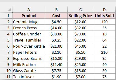
Below I have products in A, costs in B, selling prices in C, and units sold in D. I want one overall margin for these sales.
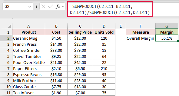
You can enter this formula in G2, beside the Overall Margin label.
=SUMPRODUCT(C2:C11-B2:B11,D2:D11)/SUMPRODUCT(C2:C11,D2:D11)
How does this formula work?
I use SUMPRODUCT to multiply corresponding values and add the results. In the first part, you multiply each product’s profit per unit by its units sold.
You add those amounts to get total profit of $6,929.
In the second SUMPRODUCT, you multiply each selling price by its units sold and add them together. You get total revenue of $12,565.
You then divide $6,929 by $12,565 to get an overall margin of 55.1%.
For comparison, you can enter this formula in G3, beside Average of Item Margins.
=AVERAGE((C2:C11-B2:B11)/C2:C11)
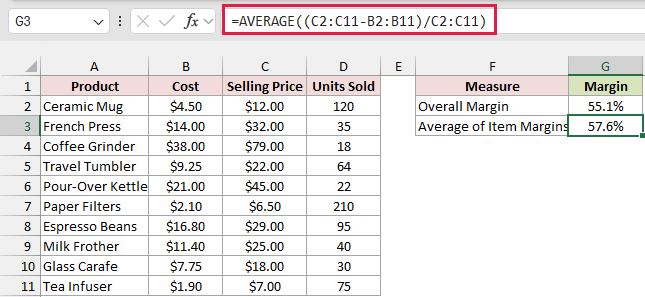
You get 57.6% from the average, which overstates your overall margin.
With that average, you give equal importance to 18 Coffee Grinders and 210 packs of Paper Filters, despite their different sales volumes.
You also ignore how much revenue each product contributes. Espresso Beans has the lowest margin, 42.1%, and is one of your biggest sellers by revenue.
I’d use the SUMPRODUCT version whenever sales volumes differ, so your overall margin reflects the sales you actually made.
Additional Notes About Margin Formulas in Excel
I keep these points in mind when building a pricing sheet so the percentages stay clear and usable.
- Label your columns “Margin” or “Markup” clearly. Mixing them up is the most common pricing mistake because you divide profit by different amounts.
- Keep percentages as real numbers formatted as %. When you type 40% into a cell, Excel stores 0.4, which is exactly what these formulas expect.
- With positive costs and selling prices, your margin always stays below 100%; markup has no upper limit. You can reach a 100% margin only when cost is zero.
- You need Excel 365 or 2021 for the spilling formulas. In older versions, use the single-cell versions and copy them down to calculate each row.
Frequently Asked Questions
Let me answer a few pricing questions where the difference between margin and markup can change your result.
Is a 50% markup the same as a 50% margin?
No. You get a 33.3% margin from a 50% markup, while you need a 100% markup to get a 50% margin.
What is the formula for profit margin percentage in Excel?
You can use =(C2-B2)/C2 when B2 contains cost and C2 contains selling price. Apply Percent Style on the Home tab to display the percentage.
How do I calculate a price after adding a 30% margin?
You can use =Cost/(1-30%). With a $100 cost, you need a $142.86 selling price for a 30% margin.
If you charge $130 instead, you’re adding a 30% markup. You’d get only a 23.1% margin.
Can a profit margin be negative?
Yes. If your cost is $10 and your selling price is $8, you get a -25% margin because you’re selling at a loss.
Conclusion
I keep one rule in mind when pricing products. You divide profit by selling price for margin, and by cost for markup.
When you have a target margin, use Cost/(1-Margin) to find the selling price that leaves you the share of profit you want.
Other Excel articles you may also like:
