
Calculating a percentage in Excel always comes down to a division or a multiplication. The hard part is knowing which number goes where.
“What share of the total is this?” needs a different formula than “how much did this grow?” or “what’s 15% of this price?”
Pick the wrong one and Excel still returns a number. It just answers a different question.
The other thing to know is that Excel stores 25% as 0.25. The percent sign is just formatting on top of the number.
In this article, I’ll show you how to find a share of a total, calculate percentage change, and increase or decrease a value by a percentage.
I’ll also show you how to work back to the original number when all you have is the result.
Here’s a quick way to pick the formula you need:
| What you want to know | Formula | Example |
|---|---|---|
| What percentage is the part of the total? | =Part/Total | 18 of 24 invoices is 75% |
| What share of a grand total is each row? | =Value/$Total$ | 1,530 of 8,500 orders is 18% |
| By what percentage did it change? | =(New-Old)/Old | 820 to 910 is an 11.0% increase |
| What is a percentage of an amount? | =Amount*Rate | 15% of $48 is $7.20 |
| Increase a value by a percentage | =Amount*(1+Rate) | $62,000 plus 4% is $64,480 |
| Decrease a value by a percentage | =Amount*(1-Rate) | $48 minus 15% is $40.80 |
| What was the original value? | =Result/(1-Rate) | $80 after 20% off was $100 |
Method #1: Dividing the Part by the Total
When you want to know what percentage one number is of another, divide the part by the total. This is the formula I reach for most often.
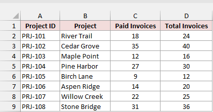
Below I have a list of projects on the Part of Total sheet. Column C has the paid invoices and column D has the total invoices.
I want the paid share of each project in column E.
Enter this formula in E2 and copy it down to E9:
=C2/D2
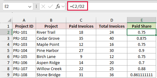
For River Trail, 18 of 24 invoices are paid, so the formula returns 0.75. That’s the right answer, just not in percentage form yet.
How does this formula work?
Excel divides the paid invoices by the total invoices in the same row. When you copy the formula down, both references move with it.
To show these decimals as percentages, apply the Percent Style format.
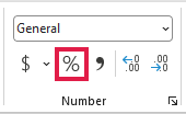
- Select E2:E9, go to the Home tab, and click the Percent Style (%) button in the Number group. On Windows, you can also press Ctrl + Shift + %.
The shares now show as percentages, like 75% for River Trail and 90% for Pine Harbor.
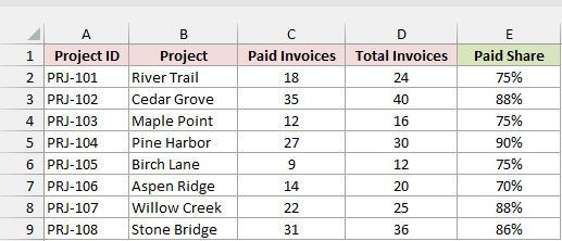
Percent Style shows whole numbers only. Cedar Grove shows 88%, but the cell still holds 0.875.
If you want to see 87.5%, click Increase Decimal in the same group.
Note: In Excel 2021, Excel 2024, and Microsoft 365, you can enter =C2:C9/D2:D9 in E2 instead. It divides every row in one go and spills the results down the column.
Method #2: Dividing by a Locked Grand Total
Sometimes each row is part of one grand total, and you want every row’s share of it. It’s still a division, but the total has to stay fixed.
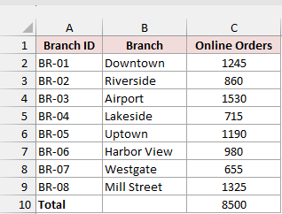
Below I have online orders by branch on the Share of Total sheet. Row 10 holds the total, calculated with =SUM(C2:C9), which gives 8,500 orders.
Enter this formula in D2 and copy it down to D10:
=C2/$C$10
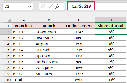
Downtown’s 1,245 orders are 15% of the total, and Airport’s 1,530 orders are 18%.
The Total row shows 100%, which is a quick check that the shares add up.
How does this formula work?
C2 is the branch’s orders and $C$10 is the grand total. The dollar signs lock C10 in place.
When you copy the formula down, C2 changes to C3, C4, and so on, but $C$10 stays the same.
Without the dollar signs, =C2/C10 turns into =C3/C11 in the next row. C11 is empty, so you get a #DIV/0! error.
To add the dollar signs quickly, click on C10 inside the formula bar and press F4.
Note: In Excel 2021, Excel 2024, and Microsoft 365, =C2:C9/C10 in D2 spills all eight shares at once. It doesn’t need dollar signs because the formula is never copied.
Method #3: Dividing the Change by the Old Value
This is the percentage increase (or decrease) formula. You subtract the old value from the new one, then divide by the old value.
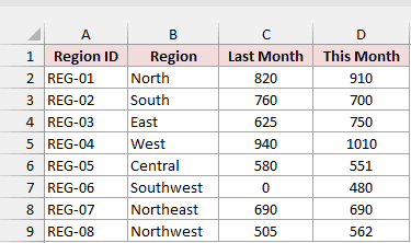
Below I have last month’s and this month’s sales for eight regions on the Percentage Change sheet. I want the percentage change in column E.
Enter this formula in E2 and copy it down to E9:
=(D2-C2)/C2
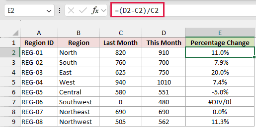
North went from 820 to 910, which shows as 11.0%. South dropped from 760 to 700, so it shows -7.9%.
A negative result means the value went down.
How does this formula work?
D2-C2 gives the change (90 for North). Dividing it by C2 turns that change into a share of where you started.
The brackets matter. Without them, Excel would divide C2 by C2 first.
Now look at Southwest. It had 0 sales last month, so the formula tries to divide by zero and returns #DIV/0!.
A change from zero can’t be expressed as a percentage, so it’s better to label it. Enter this formula in F2 and copy it down to F9:
=IF(C2=0,"n/a",(D2-C2)/C2)
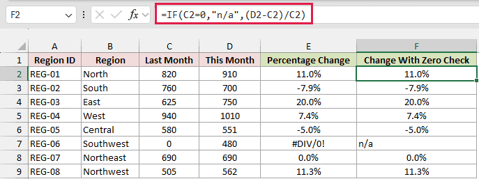
The IF function checks whether last month is 0. If it is, you get “n/a”.
If not, it runs the same percentage change formula, so every other row matches column E.
You could also use =IFERROR((D2-C2)/C2,"n/a"). It works here, but it hides every error, not just the divide-by-zero one.
When there’s no clear old and new value (say, two quotes from different suppliers), you probably want percentage difference instead, which uses a different base.
Method #4: Using the Previous Row as the Old Value
If your values are listed in time order, you can calculate the change from one period to the next by pointing the formula at the row above.
Below I have monthly revenue from January to August on the Monthly Change sheet. I want the month-over-month change in column C.
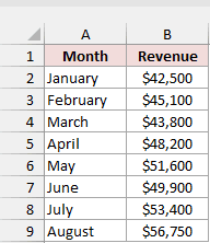
January has no previous month, so the formula starts in row 3. Enter this formula in C3 and copy it down to C9:
=(B3-B2)/B2
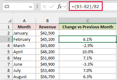
February’s revenue is 6.1% higher than January’s. March shows -2.9% because revenue dipped from $45,100 to $43,800.
How does this formula work?
It’s the same change formula from the previous method. The new value is the current row (B3) and the old value is the row above it (B2).
You may also want to compare every month against a fixed starting point. For that, lock the old value with dollar signs.
Enter this formula in D3 and copy it down to D9:
=(B3-$B$2)/$B$2
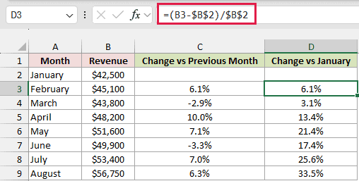
Now every month is measured against January. March is 3.1% above January even though it dropped from February, and August is 33.5% above January.
The same idea works for yearly numbers, which is how you’d calculate year-over-year growth.
Method #5: Multiplying an Amount by a Percentage
Here’s a different question. Instead of finding a percentage, you already have one and want to know how much it’s worth, like 15% of a $48 price.
Below I have a list of items on the Discounts sheet. Column C has the price and column D has the discount rate.
I want the discount amount in column E.
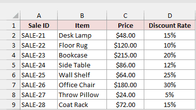
Enter this formula in E2 and copy it down to E9:
=C2*D2
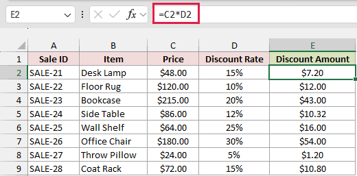
The Desk Lamp costs $48 and has a 15% discount, so the formula returns $7.20.
How does this formula work?
D2 shows 15%, but Excel stores it as 0.15. Multiplying $48 by 0.15 gives the discount amount of $7.20.
Note: Enter the rate as 15% (or 0.15 and then apply the percentage format). If you type a plain 15, Excel multiplies by 15 and the Desk Lamp discount comes out as 720 instead of 7.20.
Method #6: Multiplying by 1 Plus the Percentage
To add a percentage to a value in one step, multiply it by 1 plus the percentage.
This is how you’d work out a price increase or a salary raise.
Below I have employees on the Raises sheet. Column C has the current salary and column D has each person’s raise.
I want the new salary in column E.
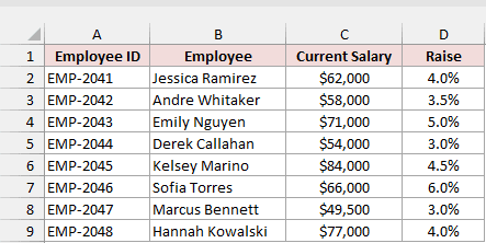
Enter this formula in E2 and copy it down to E9:
=C2*(1+D2)
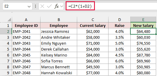
Jessica Ramirez earns $62,000 and gets a 4% raise, so her new salary is $64,480.
How does this formula work?
1+D2 is 1.04, which is the same as 104%. Multiplying the salary by 104% keeps the full salary and adds the 4% on top in a single formula.
Method #7: Multiplying by 1 Minus the Percentage
To subtract a percentage from a value, flip the sign and multiply it by 1 minus the percentage.
The most common use is working out a sale price after a discount.
Below I have the same list on the Discounts sheet, with the discount amount from Method #5 already in column E.
I want the sale price in column F.
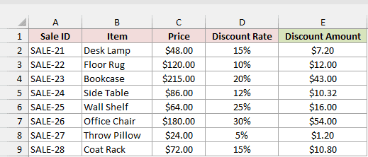
Enter this formula in F2 and copy it down to F9:
=C2*(1-D2)
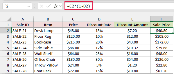
The Desk Lamp drops from $48 to $40.80 after its 15% discount.
How does this formula work?
1-D2 is 0.85, or 85%. If you take 15% off, you pay the remaining 85% of the price.
You could also subtract the discount amount (=C2-E2) and get the same $40.80. The advantage of =C2*(1-D2) is that it doesn’t need the extra column.
Method #8: Dividing by 1 Minus the Percentage
This one works backward. You know the sale price and the discount rate, and you want the original price before the discount.
Below I have orders on the Original Price sheet. Column C has the price paid and column D has the discount that was applied.
I want the original price in column E.
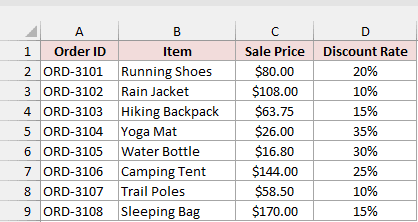
Enter this formula in E2 and copy it down to E9:
=C2/(1-D2)
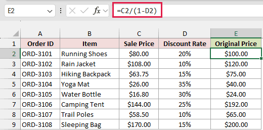
The Running Shoes sold for $80 after a 20% discount, so the original price was $100.
How does this formula work?
After a 20% discount, the $80 you paid is 80% of the original price. Dividing $80 by 0.8 (which is 1-D2) gets you back to the full $100.
A common mistake is to add the 20% back instead. =C2*(1+D2) gives $96, not $100, because the 20% is now taken from the smaller $80.
The same idea backs sales tax out of a total. If a price includes tax, divide it by 1 plus the tax rate.
For example, a $108 total that includes 8% tax started out as $100.
Additional Notes About Calculating Percentage in Excel
Most percentage problems come from a handful of mistakes. Here’s what each one looks like, so you can spot it quickly:
- You see 7500% instead of 75%. The formula multiplies by 100 (
=C2/D2*100) and the cell also has Percent Style. Drop the*100and let the format do the work. - You see 133% instead of 75%. The part and total are swapped (
=D2/C2). The part always goes on top. - Every row after the first shows #DIV/0!. The total isn’t locked. Use $C$10 so the reference doesn’t slide down into empty cells.
- A discount comes out 100 times too big. The rate was typed as 15 instead of 15%, so Excel multiplies by 15.
- Your shares add up to more than 100%. Some numbers are stored as text, so SUM skips them and the total comes out too small. Convert them to numbers first.
Frequently Asked Questions
Here are answers to a few common questions about calculating percentages in Excel.
How Do I Calculate 5% of a Number in Excel?
Multiply the number by 5%. For example, =C3*5% returns 6 for the $120 Floor Rug on the Discounts sheet.
Excel reads 5% as 0.05, so you don’t need to divide by 100.
Is There a PERCENTAGE Function in Excel?
No, there’s no function called PERCENTAGE, since a percentage is just a division.
Microsoft 365 does have the PERCENTOF function. On the Share of Total sheet, =PERCENTOF(C2,C2:C9) returns the same share for Downtown as Method #2.
Why Don’t My Percentages Add Up to 100%?
It’s usually rounding. On the Share of Total sheet, the whole-number shares you see add up to 101%.
The stored values add up to exactly 100%, which is what the Total row shows.
What Is the Difference Between a Percentage and Percentage Points?
If a paid share rises from 20% to 25%, it rose by 5 percentage points. Relative to the starting 20%, that’s a 25% increase.
Conclusion
Most percentage formulas in Excel either divide to find a percentage or multiply to apply one. Getting the right number in the denominator is most of the work.
If you’re not sure where to start, go with Method #1. Divide the part by the total, then apply Percent Style.
I hope you found this article helpful.
Other Excel articles you may also like:
- Percentage Calculator
- How to Multiply Percentages in Excel
- How to Divide in Excel
- How to Calculate Average Percentage in Excel
- Convert Number to Percentage in Excel
- Percentage Difference Calculator
- Discount Calculator
- How to Calculate Cumulative Percentage in Excel?
- Pie Chart With Percentage Labels
- Profit Margin and Markup
