Order of Operations in Excel

Excel follows a fixed order when calculating your formula, so reading it straight from left to right can lead you to expect the wrong answer.

That’s why =5+2*3 returns 11, rather than 21.

Parentheses let you tell Excel which part to calculate first, including when you’re averaging scores or increasing a price by a percentage.

I’ll show you how that order works, explain two surprises involving powers, and walk you through checking a calculation with Evaluate Formula and F9.

Excel’s Order of Operations (Operator Precedence)

A symbol that tells Excel what to do, such as + for addition, is called an operator.

The rule deciding which instruction happens first is called precedence. You can read Excel’s order from the top of this table down.

Order	Operator	What It Does	Example
1	: (colon)	Creates a range	=SUM(A1:A5)
1	Single space	Returns the cells two ranges share (intersection)	=SUM(A1:C3 B2:D4)
1	, (comma)	Combines ranges (union)	=SUM(A1:A3,C1:C3)
2	-	Makes a number negative (negation)	=-5
3	%	Percent	=20%
4	^	Exponent (power)	=2^3
5	* and /	Multiplication and division	=6*2/3
6	+ and -	Addition and subtraction	=10+5-3
7	&	Joins text (concatenation)	="Q"&1
8	= < > <= >= <>	Comparison	=A1>100

You can override this order with parentheses. Excel calculates what’s inside them first, then uses that result in the rest of your formula.

When operators share a row in the table, Excel works through them from left to right.

You may recognize this as close to PEMDAS or BODMAS from school math. I’ll cover the two differences involving powers below.

How Excel Works Through a Formula

Take the formula from earlier:

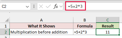
=5+2*3

You’ll get 11 because Excel multiplies 2*3 first, returning 6, and then adds 5.

If you worked straight from left to right, you’d add 5 and 2 first, then multiply 7 by 3, expecting 21.

Below I have a small table with the description in column A, the formula in column B, and the result in column C.

Using Parentheses to Change the Order

To add 5 and 2 before multiplying, I put the addition inside parentheses:

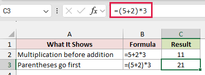
=(5+2)*3

You’ll now get 21. Excel adds 5+2 first, returning 7, then multiplies that result by 3.

Below I’ve added a second row to the small table so you can compare the formulas and their results.

Now let’s use parentheses for something you’d actually calculate: the average of a student’s two test scores.

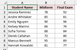
On the Test Scores sheet, I have eight students in A1:C9, with the headers Student Name, Midterm, and Final Exam.

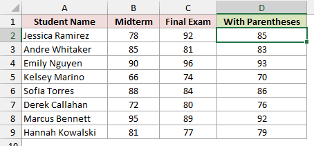
Below you can see their names and two scores. Jessica Ramirez’s row has 78 in B2 and 92 in C2.

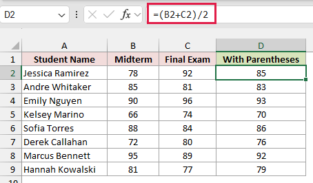
Enter With Parentheses in D1. In D2, enter this formula and copy it down to D9:

=(B2+C2)/2

How does this formula work?

Here I want Excel to add both scores before dividing. The parentheses make it calculate 78+92, returning 170, then divide by 2.

You’ll get 85 for Jessica. From D2 to D9, you’ll see 85, 83, 93, 70, 86, 76, 92, and 79.

To see the mistake, enter Without Parentheses in E1. In E2, enter this formula and copy it down to E9:

=B2+C2/2

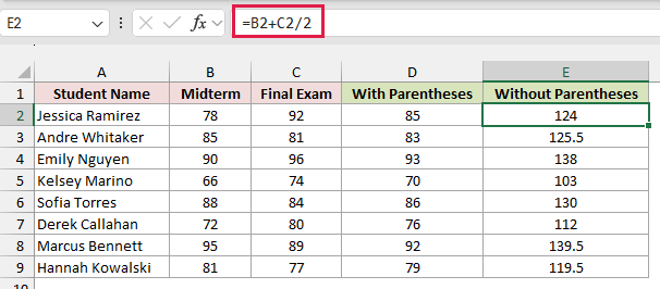
Without parentheses, you’ll get 124 for Jessica. Excel divides her final exam score, 92, by 2 first, then adds 78 to 46.

From E2 to E9, you’ll see 124, 125.5, 138, 103, 130, 112, 139.5, and 119.5.

An average higher than both original scores is your giveaway that the calculation went wrong.

I’m using a regular formula copied down here, rather than a formula that fills multiple cells automatically, to keep the focus on parentheses.

Note: When you put parentheses inside another pair, Excel starts with the innermost pair. Excel colors matching pairs as you type, which helps you check them.

Operators With the Same Precedence Go Left to Right

Multiplication and division share a level, as do addition and subtraction. Excel works through operators on the same level from left to right.

I’ve collected four examples below. Column A describes each calculation, column B shows the formula, and column C shows the result.

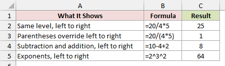
With =20/4*5, Excel divides 20 by 4 first, returning 5. It then multiplies 5 by 5 to get 25.

With =20/(4*5), Excel calculates 4*5 first. It then divides 20 by that result, 20, returning 1.

For =10-4+2, Excel subtracts 4 from 10, then adds 2. You’ll get 8, rather than 4.

Powers follow the same left-to-right rule in Excel. With =2^3^2, Excel calculates 2^3 first, returning 8, then squares 8 to get 64.

In standard math notation, you work stacked powers from the top down. That means calculating 3^2 first, then 2^9, which returns 512.

To get 512 in Excel, write =2^(3^2). The parentheses tell Excel to calculate the power on the right first.

Why =-2^2 Returns 4 in Excel

A minus sign directly in front of a number, with nothing before it, makes that number negative. This is called negation.

Excel applies that leading minus before calculating a power. When you enter =-2^2, you’ll square negative 2 and get 4.

In most math classes, you’d read -2² as the negative of 2 squared, giving -4. That’s why this Excel result can catch you out.

Below I have three examples showing how moving the minus sign or adding parentheses changes the result.

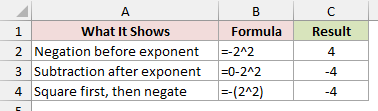
With =0-2^2, you’re subtracting from zero. Excel calculates the power first, then subtracts 4 from 0, returning -4.

With =-(2^2), you explicitly put the square first. Excel calculates 4 inside the parentheses, then makes it negative.

You’ll see the same behavior with cell references. If you put 3 in A2, =-A2^2 returns 9, while =0-A2^2 returns -9.

To square A2 first and then make the result negative, use =-(A2^2).

You can also see the rule in =-3^2+1: Excel squares negative 3, returning 9, then adds 1 for a result of 10.

Note: In =5-2^2, the minus means subtraction, so you’ll get 1 as expected. The leading minus is what behaves differently.

Watch Out for Percentages in a Formula

Parentheses also matter when you increase a price by a percentage. Here I want to raise each product’s current price by 10%.

On the Price Increase sheet, I have eight products in A1:B9, with the headers Product and Current Price.

Below you can see the products and their current prices. The Coffee Maker is in row 2, with a price of $80 in B2.

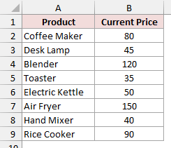
Enter With Parentheses in C1. In C2, enter this formula and copy it down to C9:

=B2*(1+10%)

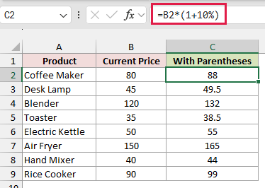
How does this formula work?

Excel reads 10% as 0.1. Inside the parentheses, you add that to 1, returning 1.1, before multiplying by the current price.

For the Coffee Maker, you’ll multiply 80 by 1.1 and get $88.

From C2 to C9, you’ll see 88, 49.5, 132, 38.5, 55, 165, 44, and 99.

Now enter Without Parentheses in D1. In D2, enter this formula and copy it down to D9:

=B2*1+10%

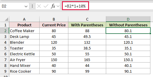
You’ll get $80.10 for the Coffee Maker. Excel multiplies 80 by 1 first, then adds 0.1.

From D2 to D9, you’ll see 80.1, 45.1, 120.1, 35.1, 50.1, 150.1, 40.1, and 90.1.

You’ve added ten cents to each price instead of increasing it by 10%. Grouping 1+10% fixes the calculation.

Where Text Joining (&) and Comparisons Fit In

You can join text with & or compare values with symbols such as >. Both sit below arithmetic in Excel’s order, so arithmetic happens first.

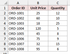
On the Order Totals sheet, I have eight orders in A1:C9, with the headers Order ID, Unit Price, and Quantity.

Below you can see those three columns. For ORD-1001 in row 2, B2 contains a unit price of $25 and C2 contains a quantity of 12.

First, I’ll create a text summary containing each order’s total. Enter Order Summary in D1, then enter this in D2 and copy it to D9:

="Total: $"&B2*C2

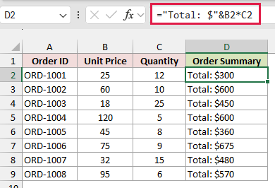
How does this formula work?

You multiply the unit price by the quantity first. Excel then joins that result to the text Total: $, so you don’t need parentheses.

For ORD-1001, you’ll get Total: $300, because 25*12 returns 300.

From D2 to D9, you’ll see these summaries:

• Total: $300
• Total: $600
• Total: $450
• Total: $600
• Total: $360
• Total: $675
• Total: $480
• Total: $570

Next, I’ll check which totals exceed $500. Enter Over $500? in E1, then enter this in E2 and copy it to E9:

=B2*C2>500

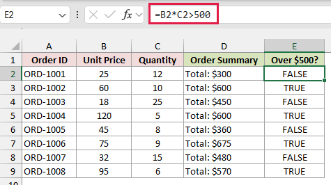
You calculate the total first, then compare it with 500. You’ll get TRUE when the total exceeds $500 and FALSE otherwise.

For ORD-1001, you’ll get FALSE because $300 isn’t above $500.

From E2 to E9, you’ll see FALSE, TRUE, FALSE, TRUE, FALSE, TRUE, FALSE, and TRUE.

How to Check the Order Excel Is Using

When you get an odd result, you can make Excel show its work. I’ll show you two ways to check which part gets calculated first.

The steps below are for Excel on Windows.

Method #1: Using the Evaluate Formula Tool

I recommend Evaluate Formula when you want to follow a calculation from beginning to end, one step at a time.

Here I’m using the Test Scores sheet, with student names in A2:A9, midterm scores in B2:B9, and final exam scores in C2:C9.

In D2:D9, I have the average formula =(B2+C2)/2 copied down. For Jessica in D2, the scores 78 and 92 produce 85.

Here are the steps to check that average:

1. Select cell D2, which contains the formula you want to check.

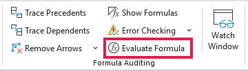
2. Go to the Formulas tab. In the Formula Auditing group, click Evaluate Formula.

You’ll see the Evaluate Formula dialog box, with your formula in the Evaluation box. The part Excel will calculate next is underlined, starting with B2.

3. Click Evaluate twice. You’ll see (78+92)/2, with 78+92 underlined for Excel to calculate next.

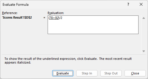
Each click replaces the underlined part with its value and underlines the next part. Here you can see Excel working inside the parentheses first.

4. Keep clicking Evaluate until you see the final result, 85, then click Close.

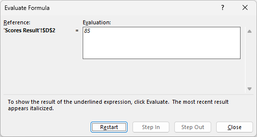
You’ll work through this sequence: (B2+C2)/2 → (78+C2)/2 → (78+92)/2 → 170/2 → 85.

If you want to follow it again, click Restart before closing the dialog box. You’ll return to the beginning of the calculation.

Method #2: Using the F9 Key

If you only want to check one part, I use F9. You select that part in the formula bar, and Excel temporarily shows its value.

Here I’m checking Jessica’s average on the Test Scores sheet. B2 contains 78, C2 contains 92, and D2 contains =(B2+C2)/2, returning 85.

Note: Press Esc afterward. If you press Enter instead, Excel keeps 170 and loses the references to B2 and C2. Press Ctrl + Z to restore them.

On a laptop, you may need Fn + F9 instead of F9.

Here are the steps to check the addition inside the parentheses:

1. Select cell D2 and click in the formula bar.

2. Select (B2+C2) and press F9. You’ll see 170 in its place, so the formula bar reads =170/2.

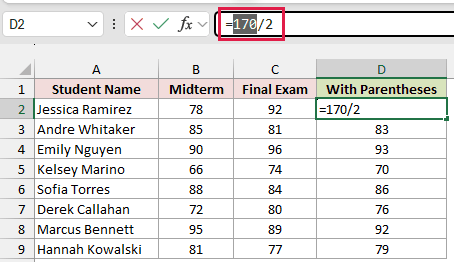
3. Press Esc to put the formula back the way it was.

Additional Notes About Order of Operations in Excel

Here are a few habits I use to keep calculations clear:

• Adding parentheses around a part Excel would calculate first anyway doesn’t change the result. It makes the formula easier to read later.
• Let a function finish before using its result. In =SUM(B2:B9)/8, Excel adds the eight values first, then divides that total by 8.
• Use parentheses to control the calculation. You can’t change Excel’s fixed order through a setting.
• Apply the same rules in conditional formatting and data validation. Their formulas follow Excel’s normal calculation order.

Frequently Asked Questions

Here are a few other questions you might have when comparing Excel with calculations elsewhere.

Why does my calculator give a different answer than Excel?

A basic four-function calculator may calculate each step as you type. That can turn 5 + 2 × 3 into 21.

In Excel, you’ll get 11 because multiplication happens first. A scientific calculator following the usual arithmetic order also returns 11.

Do spaces change the order of operations in Excel?

You can add spaces between numbers and arithmetic symbols for readability. With =5 + 2 * 3, you’ll still get 11.

A space between two cell ranges has a different job: it tells Excel to use the cells they share, called an intersection.

How do I make Excel calculate left to right?

You need to group each intended step with parentheses. Start with the leftmost calculation, then wrap that group together with the next calculation.

Keep building outward for additional steps.

Does joining numbers with & return a number or text?

You’ll get text. For example, =2+3&4 returns the text 54, rather than a numeric sum of all three values.

Excel adds 2 and 3 first, then joins 5 with 4. Use + when you want addition and & when you want joined text.

Conclusion

Excel follows a fixed order, so I use parentheses whenever I need to make the intended calculation clear.

If you’re unsure why you got a particular answer, I’d start with Evaluate Formula to see each step Excel takes.

I hope you found this article helpful.

Other Excel articles you may also like:

• How to Divide in Excel