Remove Old Items or Blanks From a Slicer in Excel

If your slicer keeps showing items you deleted from the data, or a (blank) button nobody asked for, the problem sits in the PivotTable behind it.

Refreshing doesn’t always help. Excel remembers deleted items on purpose, and a (blank) button can come from two different places in your data.

In this article, I’ll show you how to clear old items with the PivotTable’s retain setting, hide them with Slicer Settings, and fix every PivotTable at once with VBA.

I’ll also show you how to get rid of (blank) buttons for good.

How to Remove Old Items From a Slicer

The most common complaint is a slicer that still lists something you removed from the data.

Below I have 14 orders from an ice cream shop in an Excel Table. The PivotTable adds up the sales for each flavor, and the Flavor slicer filters it.

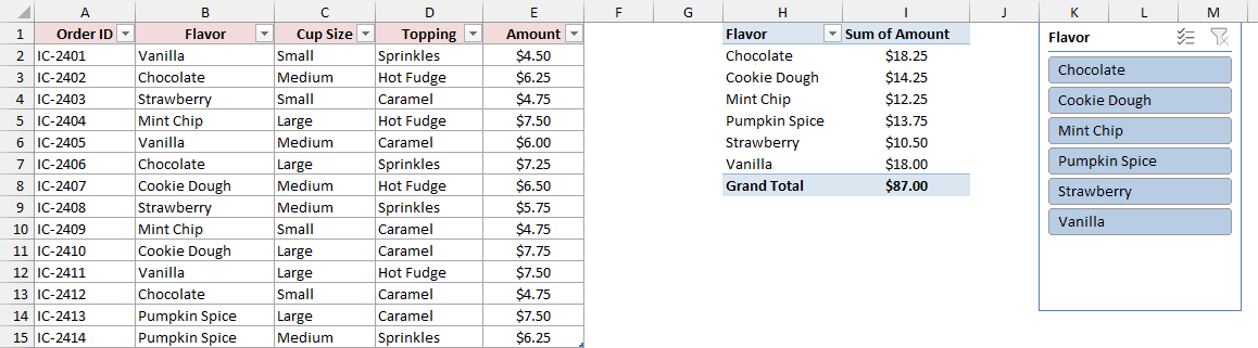
The shop stopped selling Pumpkin Spice, so I deleted its two orders and refreshed the PivotTable.

The PivotTable is correct now. It lists five flavors and a total of $73.25. But Pumpkin Spice is still in the slicer, faded and pushed to the bottom.

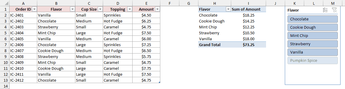
This happens because a PivotTable doesn’t read your data directly. It works from a copy called the PivotTable cache.

When you delete an item from the data and refresh, the numbers update, but the cache keeps that item’s name by default.

The slicer reads its buttons from the same cache, so the deleted item stays there too.

Method #1: Changing the Number of Items to Retain per Field (Recommended)

This is the fix I’d use in most cases. It tells the PivotTable to forget deleted items, so they leave the slicer and the PivotTable’s own filter lists.

Below I have the same ice cream orders after I deleted the two Pumpkin Spice orders. The slicer still shows a faded Pumpkin Spice button.

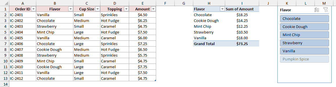
Here are the steps to remove the old item:

1. Right-click any cell in the PivotTable and choose PivotTable Options.

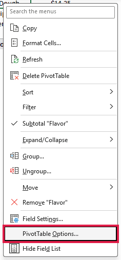
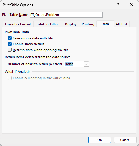
2. Go to the Data tab. In the Number of items to retain per field drop-down, choose None and click OK.

3. Right-click the PivotTable and choose Refresh (or press Alt + F5).

Pumpkin Spice is gone from the slicer. It’s also gone from the Flavor filter drop-down in the PivotTable.

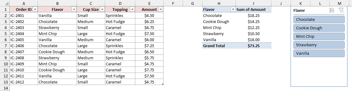
The default for this setting is Automatic, which is why old items stick around.

The refresh matters too. Changing the setting alone doesn’t clear anything until the PivotTable reloads its data.

Note: This setting belongs to the PivotTable’s cache, not to the whole workbook. PivotTables that share the cache (for example, a copied PivotTable) get fixed together. A PivotTable with its own cache needs its own change.

Method #2: Turning Off Show Items Deleted From the Data Source

If you only care about what the slicer shows, there’s a checkbox for exactly this in Slicer Settings.

Below I have the ice cream orders with Pumpkin Spice deleted. The PivotTable is right, but the slicer still has a faded Pumpkin Spice button.

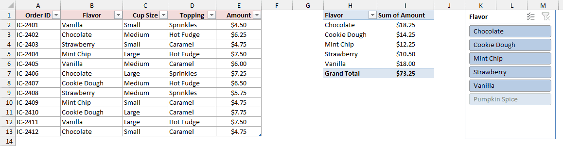
Here are the steps to hide the deleted item in the slicer:

1. Right-click the slicer and choose Slicer Settings. Uncheck Show items deleted from the data source and click OK.

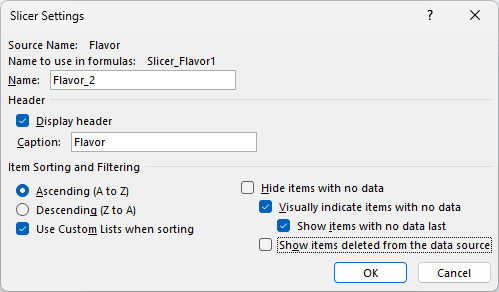
The Pumpkin Spice button disappears from the slicer.

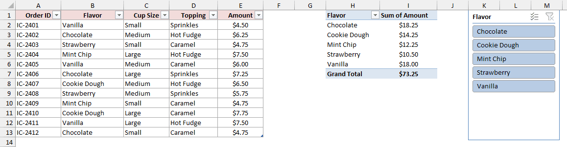
This only changes the slicer, though. The item is still in the PivotTable cache, so it still shows up in the PivotTable’s Flavor filter drop-down.

Method #1 removes it from both places.

Note: Checking Hide items with no data in the same dialog also hides the deleted item. But it hides every button that has nothing to show, including buttons that another slicer’s selection has faded out.

Method #3: Changing the Default Layout for New PivotTables

Methods #1 and #2 fix one PivotTable at a time. If you’d rather never deal with old items again, you can make None the default for every new PivotTable.

This option is in Excel for Windows with Microsoft 365 or Excel 2019 and later.

Here are the steps to change the default:

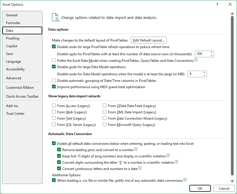
1. Go to File > Options. Click Data on the left, then click Edit Default Layout.

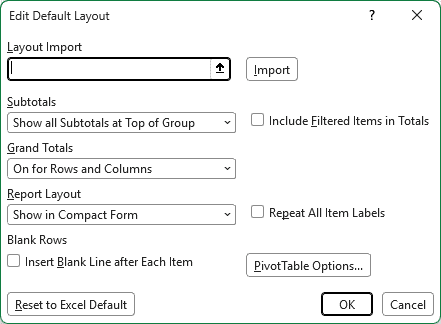
2. In the Edit Default Layout dialog box, click PivotTable Options.

3. On the Data tab, set Number of items to retain per field to None. Click OK in each open dialog box to close them.

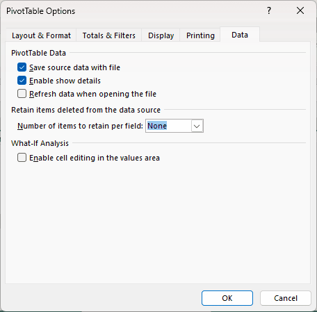
Every PivotTable you create from now on starts with None, so deleted items leave its slicers on the next refresh.

Existing PivotTables keep their current setting. Use Method #1 or Method #4 for those.

One catch: if you build a new PivotTable from the same data as an existing one in that workbook, Excel may reuse the existing cache. The new PivotTable then keeps the old setting.

Method #4: Using a VBA Macro for Every PivotTable

If a workbook has lots of PivotTables, changing each one by hand gets old fast. A short macro can set every PivotTable to None and refresh it in one go.

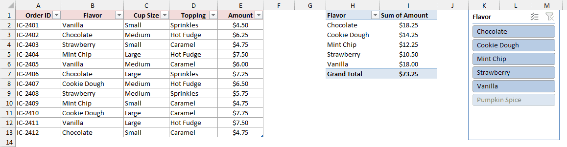
Below I have the ice cream orders with the deleted Pumpkin Spice still showing in the slicer.

Here is the VBA code:

Sub RemoveOldPivotItems()
    Dim ws As Worksheet
    Dim pt As PivotTable
    For Each ws In ActiveWorkbook.Worksheets
        For Each pt In ws.PivotTables
            pt.PivotCache.MissingItemsLimit = xlMissingItemsNone
            pt.PivotCache.Refresh
        Next pt
    Next ws
End Sub

Sub RemoveOldPivotItems()
    Dim ws As Worksheet
    Dim pt As PivotTable
    For Each ws In ActiveWorkbook.Worksheets
        For Each pt In ws.PivotTables
            pt.PivotCache.MissingItemsLimit = xlMissingItemsNone
            pt.PivotCache.Refresh
        Next pt
    Next ws
End Sub

Here are the steps to use this macro:

1. Press Alt + F11 to open the VBA editor.
2. Go to Insert > Module and paste the code into the new module.
3. Click anywhere inside the code and press F5 to run it.

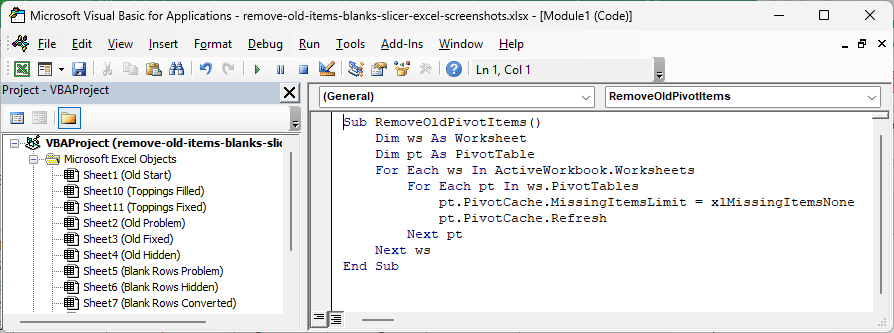
The macro goes through every worksheet in the active workbook and every PivotTable on it.

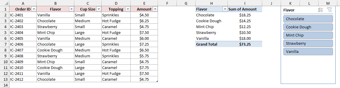
For each one, it sets the retain setting (MissingItemsLimit in VBA) to None and refreshes the cache. It’s the same change as Method #1, applied to every PivotTable.

Note: You can’t undo a macro with Ctrl + Z, so save your file first. To keep the macro in the workbook, save it as an .xlsm file.

How to Remove (blank) From a Slicer

A (blank) button means the slicer’s field has empty values somewhere in the PivotTable’s source.

There are two very different reasons for that, and the fix depends on which one you have.

Look at the (blank) button first:

• A faded (blank) button usually means the source range includes empty rows below your data. Methods #5 and #6 are for this.
• A normal, clickable (blank) button means some real rows have an empty cell in that column. Method #7 is for this.

Method #5: Using Hide Items With No Data

This is the quickest way to get a faded (blank) out of the slicer.

Below I have the 12 ice cream orders as a normal range. When I made the PivotTable, I selected whole columns A:E so new orders would be picked up.

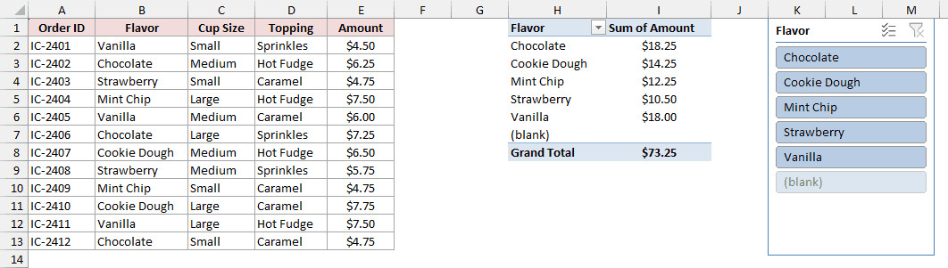
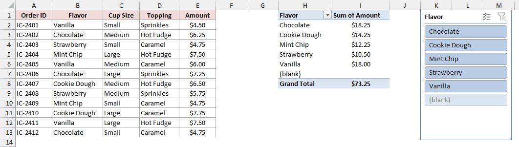
Because the source includes all the empty rows below the data, the PivotTable shows a (blank) row with no amount. The Flavor slicer has a faded (blank) button.

Here are the steps to hide it:

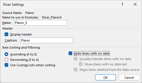
1. Right-click the slicer and choose Slicer Settings. Check Hide items with no data and click OK.

The (blank) button is gone from the slicer.

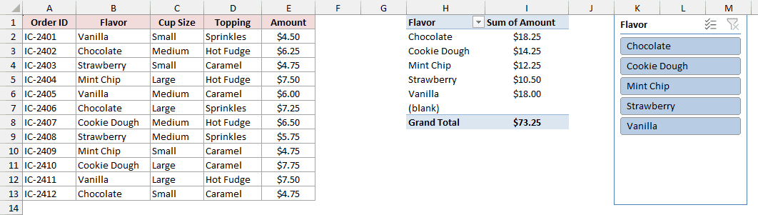
The PivotTable still has its (blank) row, though, because the empty rows are still part of the source. To fix the cause, use Method #6.

Note: Hide items with no data only removes (blank) when the button is faded. A normal (blank) button has real rows behind it, so this setting leaves it alone.

Method #6: Changing the Source to an Excel Table

An Excel Table is the cleaner way to make a PivotTable pick up new rows.

It covers only your data, and it grows by itself when you add orders, so there are no empty rows to create a (blank).

Below I have the same 12 orders, with the PivotTable built on whole columns A:E. The PivotTable has a (blank) row and the slicer has a faded (blank) button.

Here are the steps to switch the PivotTable to a Table:

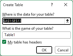
1. Click any cell in the data and press Ctrl + T. Make sure My table has headers is checked and click OK. Excel suggests a name for the Table in the same dialog (Table1 here).

2. Select any cell in the PivotTable, go to the PivotTable Analyze tab, and click Change Data Source.

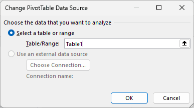
3. In the Table/Range box, type the Table’s name (Table1 here) and click OK. You can see the name on the Table Design tab.

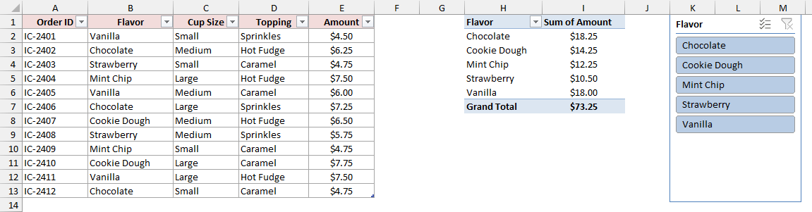
The PivotTable now reads only the 12 orders. The (blank) row is gone, and so is the (blank) button in the slicer.

If a faded (blank) button is still in the slicer after this, it’s a leftover in the PivotTable cache. Method #1 clears it.

Method #7: Filling the Blank Cells in the Source Data

When the (blank) button is normal and clickable, some real rows have an empty cell. The fix is to give those cells a proper label.

Below I have the 12 ice cream orders in an Excel Table, with a PivotTable of sales by topping.

Three plain cups have no topping, so the Topping slicer shows (blank) with $19.00 of sales.

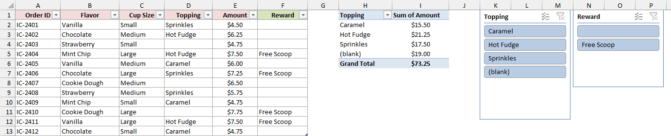
There’s a second problem in the Reward slicer. It has a button with no name at all.

That one comes from the Reward column, which uses this formula:

=IF(E2>=7,"Free Scoop","")

The formula returns an empty text string (“”) for orders under $7.

Excel doesn’t treat that as a true blank, so the slicer shows it as an empty button instead of (blank).

Here are the steps to fill the empty topping cells:

1. Select the topping cells, D2:D13.
2. Go to Home > Find & Select > Go To Special. Choose Blanks and click OK.

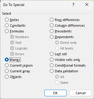
3. Only the three empty cells are selected now. Type No Topping and press Ctrl + Enter to fill all three at once.

For the Reward column, change the formula in F2 so it returns a label instead of “”, and copy it down the column:

=IF(E2>=7,"Free Scoop","No Reward")

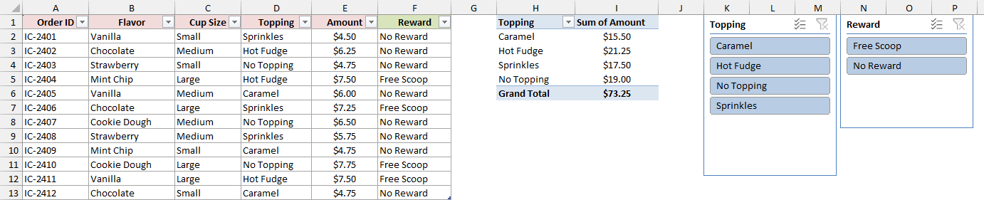
Now refresh the PivotTable. No Topping ($19.00) and No Reward show up as normal buttons.

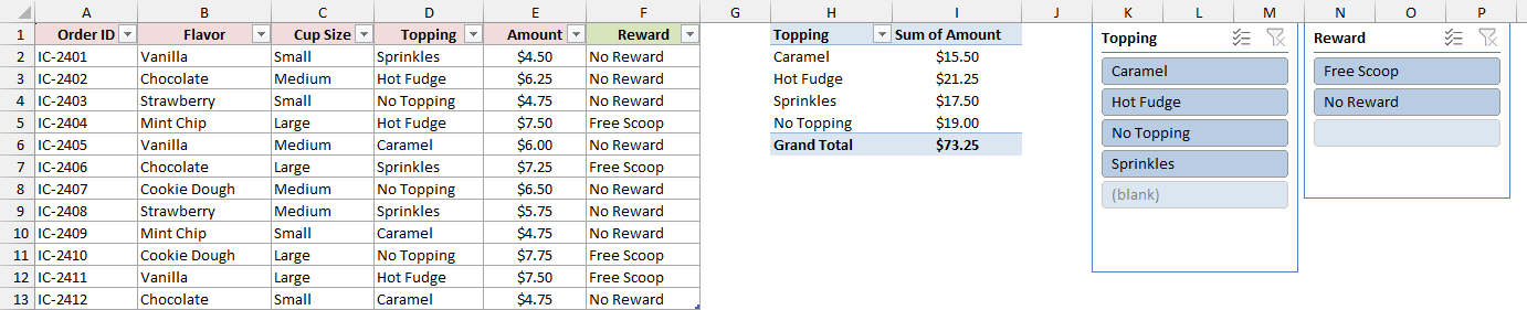
But look at the bottom of each slicer. The old (blank) and the old empty button are still there, faded.

These are leftovers in the PivotTable cache, exactly like the deleted Pumpkin Spice earlier. Set the retain setting to None with Method #1 and refresh, and both slicers are clean.

Additional Notes About Removing Old Items and Blanks From a Slicer

• Refresh after every fix. A slicer only updates when its PivotTable reloads the data, so a changed setting or a cleaned-up source shows nothing until you refresh.
• A Table source fixes the (blank) problem from empty rows, but it doesn’t stop old items. A PivotTable built on a Table still keeps deleted items until you change the retain setting.
• The retain setting is saved with the PivotTable’s cache, so anyone who opens the workbook gets the same clean slicer.
• Cleaning up the source data often leaves a faded leftover button behind. It stays until the retain setting is None.
• Each sheet in the example file is saved with the problem still showing, so you can try every fix yourself.
• The steps and shortcuts here are for Excel for Windows.

Frequently Asked Questions

Here are some questions people often ask about old items and blanks in slicers.

Do I have to fix every slicer separately?

Not with Method #1. The retain setting lives in the PivotTable cache, so every slicer on that PivotTable loses the old item after one refresh.

The Slicer Settings checkboxes in Methods #2 and #5 are different. You set those on each slicer.

Will changing the retain setting affect my other PivotTables?

Only the PivotTables that share the same cache. A PivotTable you copied from another one usually shares its cache, so it changes too. PivotTables built separately keep their own setting.

Why is “Show items deleted from the data source” greyed out?

Microsoft’s documentation says this option works only for slicers on regular worksheet data, not OLAP sources.

A Data Model (Power Pivot) PivotTable is an OLAP source, so the option isn’t available there.

Can I remove (blank) from a slicer without changing my data?

Yes, if the (blank) button is faded. Check Hide items with no data in Slicer Settings.

A normal (blank) button has real rows behind it, so you’ll need to fill those cells instead.

Conclusion

In this article, I showed you how to remove old items from a slicer with the retain setting, Slicer Settings, a new default layout, and a VBA macro.

I also showed you how to get rid of (blank) buttons by fixing the source range or filling the empty cells.

For old items, Method #1 is the one I’d use first.

I hope you found this article helpful.

Other Excel articles you may also like:

• Pivot Table Not Refreshing – How to Fix?
• How to Connect Slicer to Multiple Pivot Tables
• How to Clear Cache in Excel?
• How to Delete a Pivot Table in Excel?