Pivot Table Not Refreshing – How to Fix?

When a PivotTable does not refresh, its report can keep old totals or omit newly added records.

A basic refresh works only when Excel can read the right source and nothing blocks the update.

If the usual steps to refresh a PivotTable in Excel do not work, check the source range first.

Below, I cover nine reasons a PivotTable stays stale, starting with the most common one: new data outside the source range.

Reason #1: New Data Is Outside the Source Range

A PivotTable built from a fixed range keeps reading that same range when you refresh it. Rows added below the range remain outside its source.

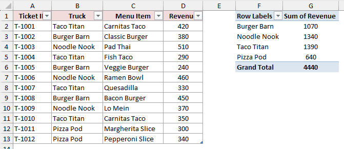
On the Reason 1 Problem sheet, the data occupies A1:D13, but the PivotTable source stops at A1:D11.

You will see Burger Barn at 1070, Noodle Nook at 1340, and Taco Titan at 1390. Pizza Pod is missing, and the Grand Total remains 3800.

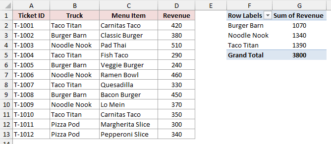
Refreshing cannot extend a fixed source range. You need to change the range or convert the source into an Excel Table.

Fix #1: Change the Data Source

Use this fix when the source range is correct apart from newly added rows or columns.

Here are the steps to include the two new rows:

1. Click any cell in the PivotTable. On the PivotTable Analyze tab, click Change Data Source.

2. Change the source to $A$1:$D$13, then click OK.

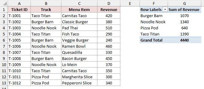
Pizza Pod now appears with revenue of 640, and the Grand Total changes to 4440.

This fix works, but you must change the range again whenever future data falls outside it.

Fix #2: Convert the Source Data to an Excel Table

An Excel Table expands as you add records. Pointing the PivotTable to that table prevents the same fixed-range problem from returning.

The Reason 1 Fix sheet shows the finished setup. Its A1:D13 range is already the Excel Table TruckSales, and the PivotTable uses that table.

To make the same change in your workbook, start with fixed-range data such as the source on Reason 1 Problem.

Here are the steps:

1. Select A1:D13 and press Ctrl+T.

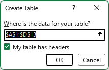
2. Confirm the range, select My table has headers, and click OK.

3. Click inside the PivotTable, choose PivotTable Analyze > Change Data Source, enter TruckSales, and click OK.

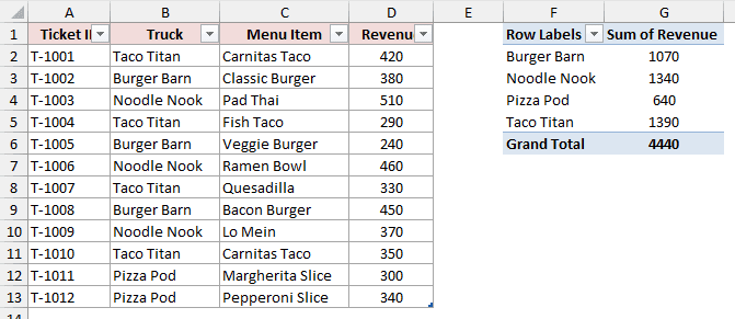
The PivotTable shows Burger Barn 1070, Noodle Nook 1340, Pizza Pod 640, Taco Titan 1390, and a Grand Total of 4440.

Note: I recommend the Excel Table fix for most readers because the source expands automatically when you add new rows.

Reason #2: Only One PivotTable Was Refreshed

Pressing Alt+F5 or choosing Refresh updates only the selected PivotTable and its cache. PivotTables built from other sources can remain stale.

For example, refreshing a sales PivotTable will not update an inventory PivotTable built from a separate source.

Fix: Use Refresh All

Refresh All updates every PivotTable and connection in the workbook instead of only the active PivotTable.

Here is how to run it:

1. Click inside a PivotTable. On the PivotTable Analyze tab, open the Refresh arrow and choose Refresh All.

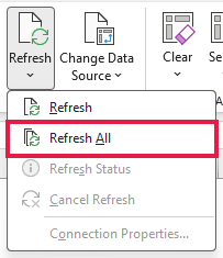
You can also press Ctrl+Alt+F5 or choose Data > Refresh All.

Reason #3: Excel Never Refreshes a PivotTable by Itself

A PivotTable does not watch its source. Edit the data and the report keeps the numbers from the last refresh.

That catches people out with a workbook they open each morning, where the source changed but the report did not.

Fix: Refresh Data When Opening the File

This setting tells Excel to refresh the PivotTable every time the workbook opens, so you start from current numbers.

Here are the steps:

1. Click inside the PivotTable and choose PivotTable Analyze > Options.

2. Open the Data tab, select Refresh data when opening the file, and click OK.

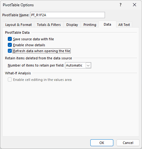
Note: This refreshes on open only. If the data changes while the workbook is open, press Alt+F5 or use Refresh All.

Reason #4: A Manual Filter Hides the New Items

A field filter created by clearing item checkboxes can keep excluding items that did not exist when you set the filter.

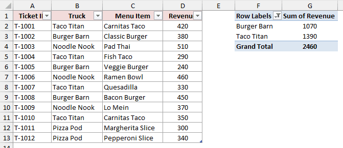
On the Reason 4 Problem sheet, the source includes Pizza Pod. The Truck field has Noodle Nook manually excluded, but Pizza Pod also remains hidden after refresh.

The PivotTable shows Burger Barn 1070 and Taco Titan 1390, with a Grand Total of 2460.

Fix: Include New Items in the Manual Filter

This setting keeps your existing exclusions while allowing newly added field items to appear after a refresh.

Here are the steps:

1. Click a Truck label. On the PivotTable Analyze tab, click Field Settings, then open the Subtotals & Filters tab.

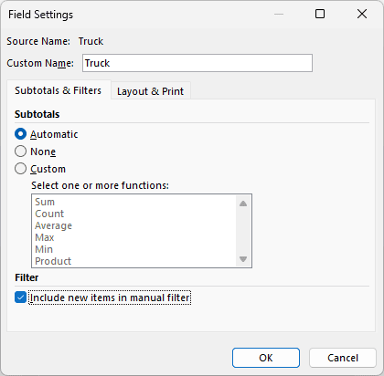
2. Select Include new items in manual filter, click OK, and refresh the PivotTable.

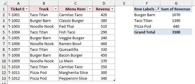
On the Reason 4 Fix sheet, Pizza Pod appears at the end of the list with 640. Noodle Nook stays filtered out, so the Grand Total becomes 3100.

Note: Include new items in manual filter is grayed out when the field is in the Filters area rather than the Rows or Columns area.

Reason #5: Calculation Is Set to Manual

A PivotTable can read stale source values when those values come from formulas and Excel’s calculation mode is set to Manual.

Refreshing the PivotTable does not force every source formula to recalculate first. You can still see an old total until the source formulas recalculate.

Fix: Recalculate Before You Refresh

Recalculate the workbook before asking the PivotTable to read the source again.

Here are the steps:

1. Press F9 to recalculate the workbook, then refresh the PivotTable.

2. For ongoing recalculation, choose Formulas > Calculation Options > Automatic.

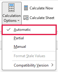
If you intentionally use Manual calculation, keep the F9 step in your refresh routine.

Reason #6: The Worksheet Is Protected

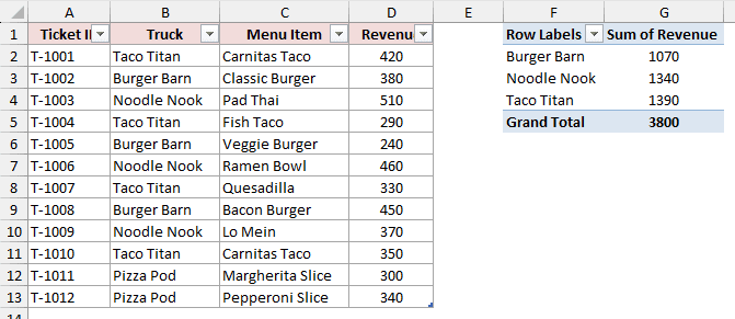
Worksheet protection can disable Refresh or make the refresh fail. On the Reason 6 sheet, the protected PivotTable still shows the old Grand Total of 3800.

The Pizza Pod rows are in the source, but the PivotTable cannot update while the sheet is protected.

Fix: Unprotect the Worksheet

Remove protection, refresh the PivotTable, and then restore protection if the sheet still needs it.

Here are the steps:

1. On the Review tab, click Unprotect Sheet. Enter the password if Excel asks for one.

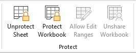
2. Refresh the PivotTable.

Pizza Pod appears with 640, and the Grand Total becomes 4440. Re-protect the worksheet afterward if needed.

Reason #7: The PivotTables Would Overlap

A PivotTable needs room to grow when a refresh adds new row or column items. Excel stops the update if that growth would touch another PivotTable.

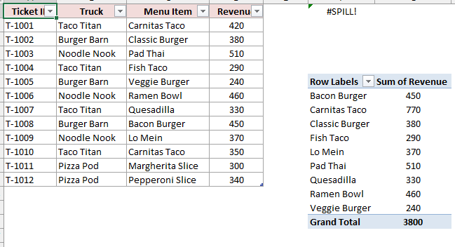
On the Reason 7 Problem sheet, the Truck PivotTable occupies F1:G5, while the Menu Item PivotTable starts directly below at F6:G16.

Adding Pizza Pod requires another row. In current Microsoft 365, the growing PivotTable shows a #SPILL! placeholder and does not update.

Older Excel versions may instead show “A PivotTable report cannot overlap another PivotTable report.”

Fix: Move One PivotTable

Leave enough blank space for both PivotTables to expand during future refreshes.

Here are the steps:

1. Click inside the lower PivotTable and choose PivotTable Analyze > Move PivotTable.

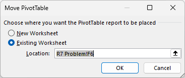
2. Set the new location to I1, or choose a new worksheet, then click OK.

3. Refresh the PivotTables.

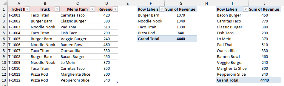
On the Reason 7 Fix sheet, the Truck PivotTable expands to F1:G6 and totals 4440. The Menu Item PivotTable sits at I1:J13 and also totals 4440.

Reason #8: A Source Column Has No Header

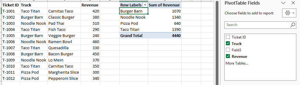
Current Microsoft 365 silently assigns a generic name such as Field3 to a source column with a blank header.

The PivotTable Fields list then shows that meaningless name, so the expected column appears to be missing. A merged header can instead shrink the source range.

Older Excel versions may show “The PivotTable field name is not valid.” The message can also appear when a new PivotTable uses a range with an invalid header row.

An all-blank header row can show “Data source reference is not valid.”

Fix: Add the Missing Header

Check the first row of the source range before refreshing again.

Here are the steps:

1. Type a unique header into every blank header cell.

2. If header cells are merged, unmerge them and give each source column its own heading.

3. Refresh the PivotTable.

Reason #9: The Data Comes From Power Query

Refreshing a PivotTable rereads its loaded source table. It does not necessarily rerun the Power Query that loads fresh records into that table.

If the query output is stale, the PivotTable can refresh successfully and still show old numbers.

Fix: Refresh the Query First

Update the query before refreshing the PivotTable, or use Refresh All to update workbook connections together.

Here are the steps:

1. Choose Data > Refresh All, or press Ctrl+Alt+F5.

2. If the numbers remain old, open Data > Queries & Connections, right-click the query, choose Refresh, and then refresh the PivotTable.

3. For recurring timing problems, right-click the query, choose Properties, and open the Usage tab.

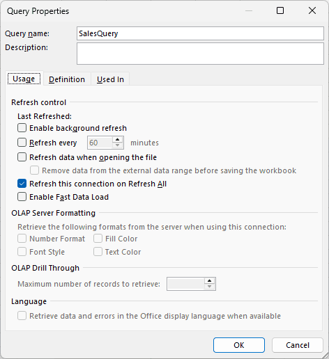
Make sure Refresh this connection on Refresh All is selected.

If Refresh All still shows old values, try clearing Enable background refresh. This can help when the PivotTable updates before the query finishes.

Additional Notes About Pivot Tables Not Refreshing in Excel

• Refresh rereads the current PivotTable source. It never expands a fixed source range by itself.
• PivotTables that share one cache can refresh together. This behavior is expected.
• To stop widths changing, open PivotTable Options > Layout & Format and clear Autofit column widths on update.
• In Excel for the web, open the Refresh All dropdown on the PivotTable tab and choose Refresh.
• New items may appear at the end of a PivotTable field after refresh until you sort that field again.
• Microsoft has been testing a PivotTable Auto Refresh button that updates the report as the source changes. It has come and gone across Microsoft 365 Insider builds with no general release date, so do not count on it.

Frequently Asked Questions

Why Is My Pivot Table Not Picking Up New Data?

Its source probably stops before the new rows. Check Change Data Source, then use the complete range or convert the source to an Excel Table.

How Do I Make a Pivot Table Refresh Automatically?

Turn on Refresh data when opening the file in PivotTable Options > Data. That is the automatic option available in every desktop version of Excel.

Why Do Deleted Items Still Show in My Pivot Table Filter?

Open PivotTable Options > Data and set Number of items to retain per field to None. Refresh the PivotTable to clear the retained items.

Why Is Refresh Grayed Out in My Pivot Table?

Click inside the PivotTable first. If Refresh remains unavailable, check whether the worksheet is protected and unprotect it before trying again.

Does Refresh All Refresh Every Pivot Table in the Workbook?

Yes. Refresh All updates every PivotTable and workbook connection, although a Power Query timing issue may require refreshing the query before the PivotTable.

Conclusion

I recommend using an Excel Table as the source because it prevents the most common problem: new rows sitting outside a fixed range.

When a refresh still leaves old results, check the matching reason above instead of repeatedly clicking Refresh.

Other Excel articles you may also like:

• Data Source Reference is Not Valid Error in Excel – Fix!
• How to Clear Cache in Excel?
• GETPIVOTDATA Function in Excel