
Slicers let anyone filter a report with one click.
But some reports only make sense for one item at a time, like a sales summary for a single store or a report for one manager.
The problem is that a slicer always lets people pick more than one item. Excel has no setting that turns this off.
Hold Ctrl, click a second button, and the report quietly adds both items together.
So the fix is a workaround. You can make multiple selections harder to do, catch them with a formula, or stop them with a short macro.
In this article, I’ll show you how to hide the slicer header, add a formula warning, and use VBA to keep only one item selected.
I’ll also cover a single-select report filter and how to set a default selection when the file opens.
Method #1: Hiding the Slicer Header
The quickest thing you can do is hide the slicer’s header. The header holds the Multi-Select button, which lets people click several items without holding any key.
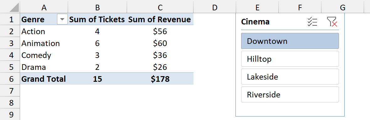
Below I have a PivotTable that shows ticket sales by genre for a chain of cinemas.
The Cinema slicer next to it filters the report, and right now Downtown is selected.
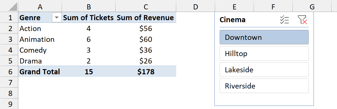
At the top of the slicer, you can see the Multi-Select button and the Clear Filter button next to the Cinema caption.
Here are the steps to hide the slicer header:
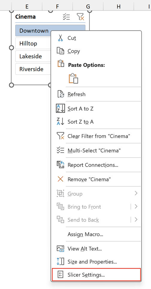
- Right-click the slicer and choose Slicer Settings.
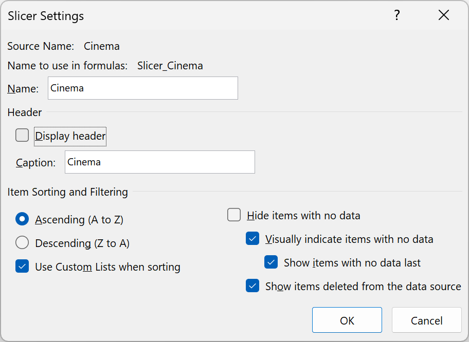
- In the Slicer Settings dialog box, uncheck Display header and click OK.
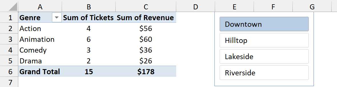
The header is gone, and so are the Multi-Select and Clear Filter buttons. Now a normal click on another cinema replaces Downtown.
This makes multiple selections harder, but it doesn’t block them. If you hold Ctrl and click another item, the slicer still selects both.
Below, I Ctrl+clicked Lakeside, and the PivotTable now adds Downtown and Lakeside together.
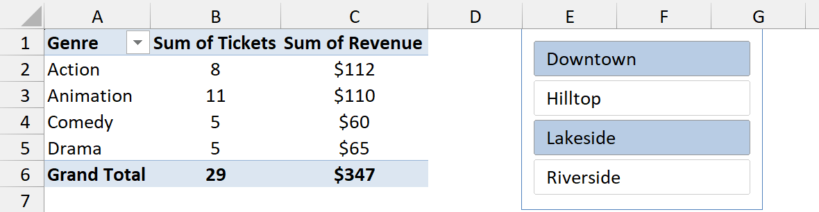
The slicer’s right-click menu also still has Multi-Select and Clear Filter, so anyone who right-clicks it can switch multi-select back on.
Note: Hiding the header also removes the slicer’s caption. If people need to know what the slicer filters, type a label like “Cinema” in the cell above it.
I’d use this method when the report is only for you or a few people who know the rule.
For anything shared more widely, pair it with the formula warning or the macro below.
Method #2: Using a Formula Warning
If you can’t stop people from picking two items, you can at least make sure they notice.
This method shows a warning and blanks out a result whenever more than one item is selected.
The trick is the PivotTable’s Filters area. When a field sits there, the PivotTable shows its current filter in a cell.
That cell reads “(Multiple Items)” when more than one item is selected, and a formula can check for it.
Below I have a PivotTable that shows tickets and revenue by genre for a chain of cinemas. The Cinema slicer next to it has Downtown selected.
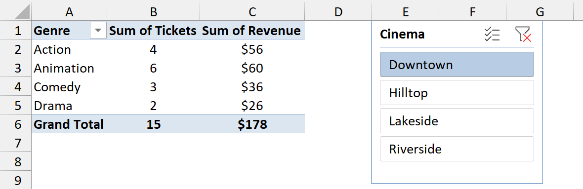
First, I’ll add the Cinema field to the Filters area. Click anywhere in the PivotTable, then drag <strong>Cinema</strong> into the <strong>Filters</strong> box in the PivotTable Fields pane.
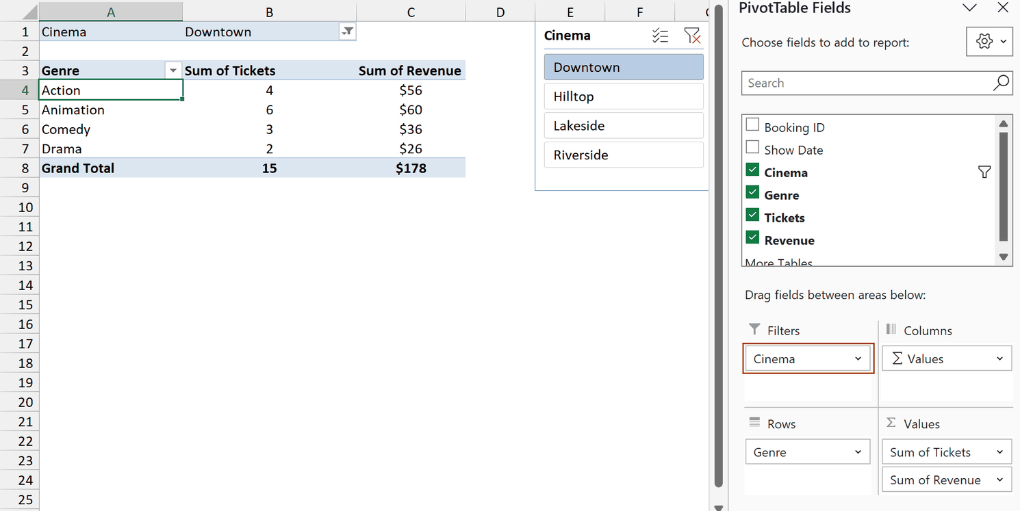
The PivotTable moves down two rows, and cell B1 now shows the slicer selection.
The slicer and this filter stay in sync, because they filter the same field.
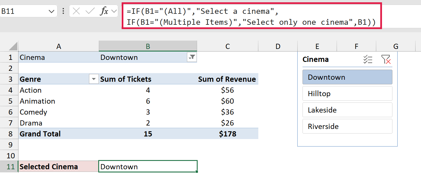
Now I’ll add a formula that tells you what’s selected. In cell B11, next to the Selected Cinema label, I entered this formula:
=IF(B1="(All)","Select a cinema",IF(B1="(Multiple Items)","Select only one cinema",B1))
How does this formula work?
The formula reads the filter cell B1. If the slicer is cleared, B1 shows “(All)”, so the formula asks you to select a cinema.
If two or more cinemas are selected, B1 shows “(Multiple Items)”, and the formula returns “Select only one cinema”. Otherwise, it returns the cinema’s name.
Next, I want to calculate the revenue per ticket, but only when one cinema is selected. In cell B12, I entered this formula:
=IF(OR(B1="(All)",B1="(Multiple Items)"),"",GETPIVOTDATA("Sum of Revenue",$A$3)/GETPIVOTDATA("Sum of Tickets",$A$3))
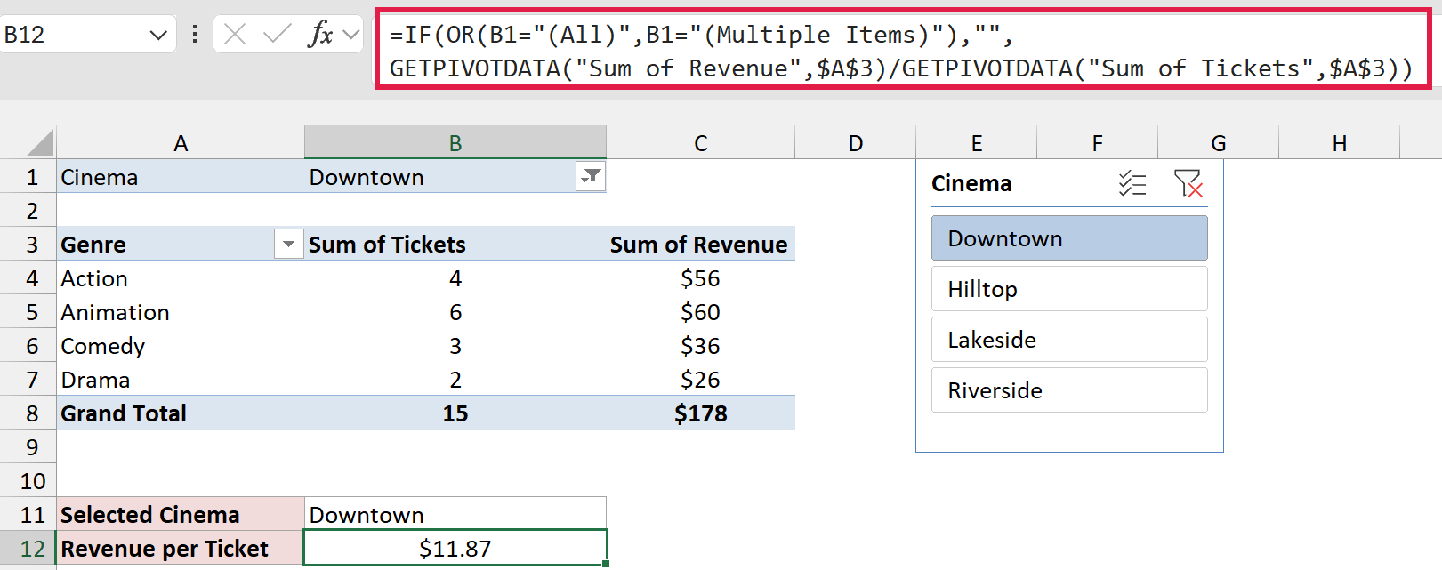
For Downtown, it returns $11.87, which is $178 in revenue divided by 15 tickets.
How does this formula work?
The GETPIVOTDATA function pulls a value out of a PivotTable.
Here, it pulls the grand totals for Sum of Revenue and Sum of Tickets, using A3 as a reference to the PivotTable.
The OR check wraps around that division. When the filter cell shows “(All)” or “(Multiple Items)”, the formula returns an empty string instead of a number.
Here’s what happens with two cinemas. Below, I Ctrl+clicked Lakeside in the slicer.
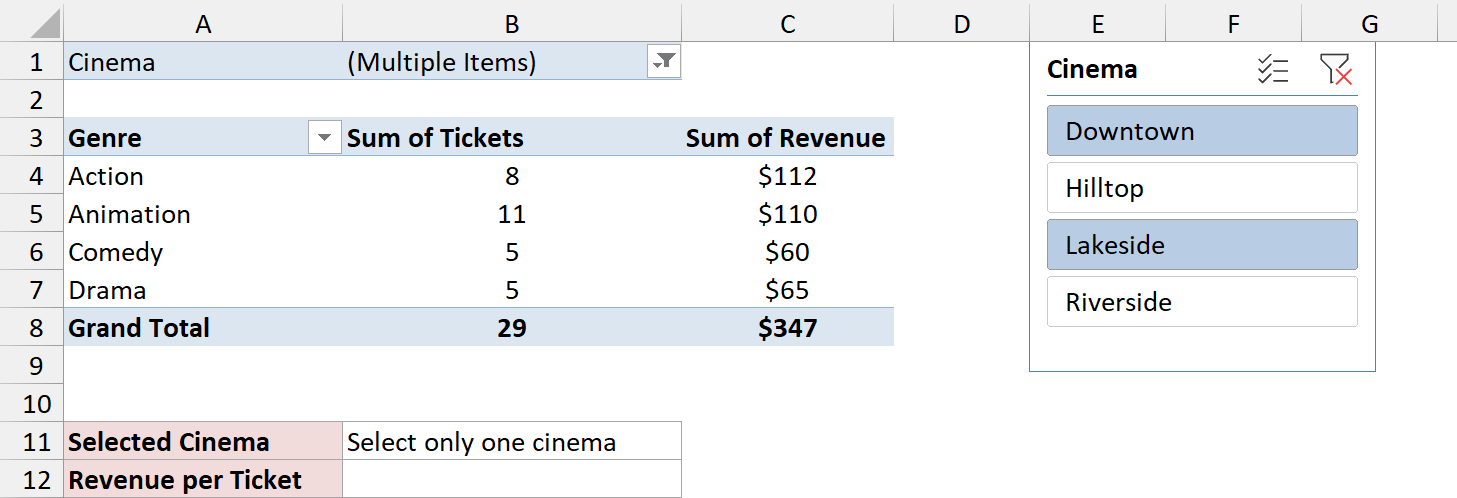
Cell B1 now reads “(Multiple Items)”, B11 shows “Select only one cinema”, and B12 is blank. So nobody mistakes the combined numbers for one cinema’s figures.
Note: If you don’t want to change your report’s layout, create a small second PivotTable with only Cinema in its Filters area. Then connect the slicer to both PivotTables and point the formulas at the second one.
This method works in any workbook, with no macros. It doesn’t stop the second selection, but it makes sure a wrong number never shows up as a real one.
Method #3: Using a VBA Macro
This is the only method that actually enforces one selection.
A short macro watches the PivotTable, and whenever a second item gets selected, it keeps the new one and turns the other off.
Below I have a PivotTable that shows tickets and revenue by genre for a chain of cinemas. The Cinema slicer next to it has Downtown selected.
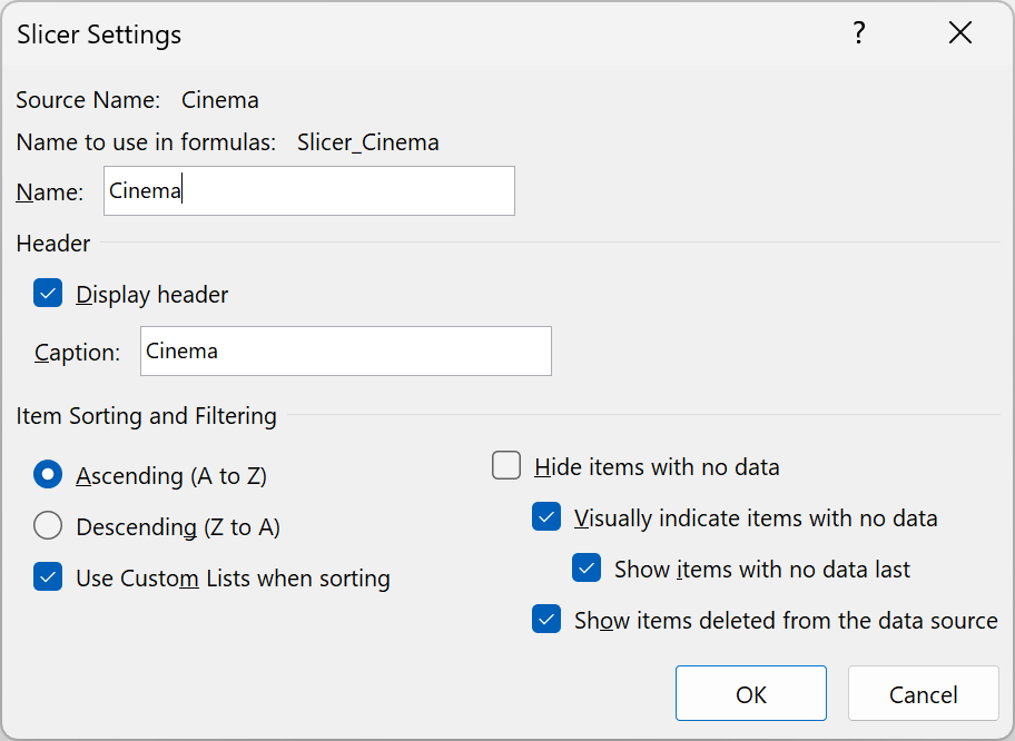
Before adding the code, you need the slicer’s name. Right-click the slicer, choose <strong>Slicer Settings</strong>, and look at <strong>Name to use in formulas</strong>. In my file, it’s Slicer_Cinema.
Here is the VBA code:
Option Explicit

' The slicer to limit. Find its name in Slicer Settings > Name to use in formulas.
Private Const SLICER_NAME As String = "Slicer_Cinema"
Private LastPick As String

Private Sub Workbook_SheetPivotTableUpdate(ByVal Sh As Object, ByVal Target As PivotTable)
    Dim sc As SlicerCache
    Dim si As SlicerItem
    Dim picked As Long
    Dim newPick As String
    Dim lastStillOn As Boolean
    Dim keep As String

    Set sc = Me.SlicerCaches(SLICER_NAME)

    For Each si In sc.SlicerItems
        If si.Selected Then
            picked = picked + 1
            If si.Name = LastPick Then
                lastStillOn = True
            ElseIf newPick = "" Then
                newPick = si.Name
            End If
        End If
    Next si

    ' Only one item selected: nothing to fix, just remember it
    If picked = 1 Then
        If newPick <> "" Then LastPick = newPick
        Exit Sub
    End If

    ' One item was added to the last pick (Ctrl+click or Multi-Select): keep the new one.
    ' Anything else (Clear Filter, dragging across items): go back to the last pick.
    If picked = 2 And lastStillOn Then
        keep = newPick
    ElseIf LastPick <> "" Then
        keep = LastPick
    Else
        keep = newPick
    End If

    On Error GoTo CleanUp
    Application.EnableEvents = False
    Application.ScreenUpdating = False
    sc.SlicerItems(keep).Selected = True
    For Each si In sc.SlicerItems
        If si.Name <> keep Then si.Selected = False
    Next si
    LastPick = keep

CleanUp:
    Application.ScreenUpdating = True
    Application.EnableEvents = True
End SubHere are the steps to add this macro:
- Press Alt + F11 to open the VBA editor.
- In the Project Explorer on the left, double-click ThisWorkbook.
- Paste the code into the code window. If your slicer has a different name, change Slicer_Cinema in the SLICER_NAME line.
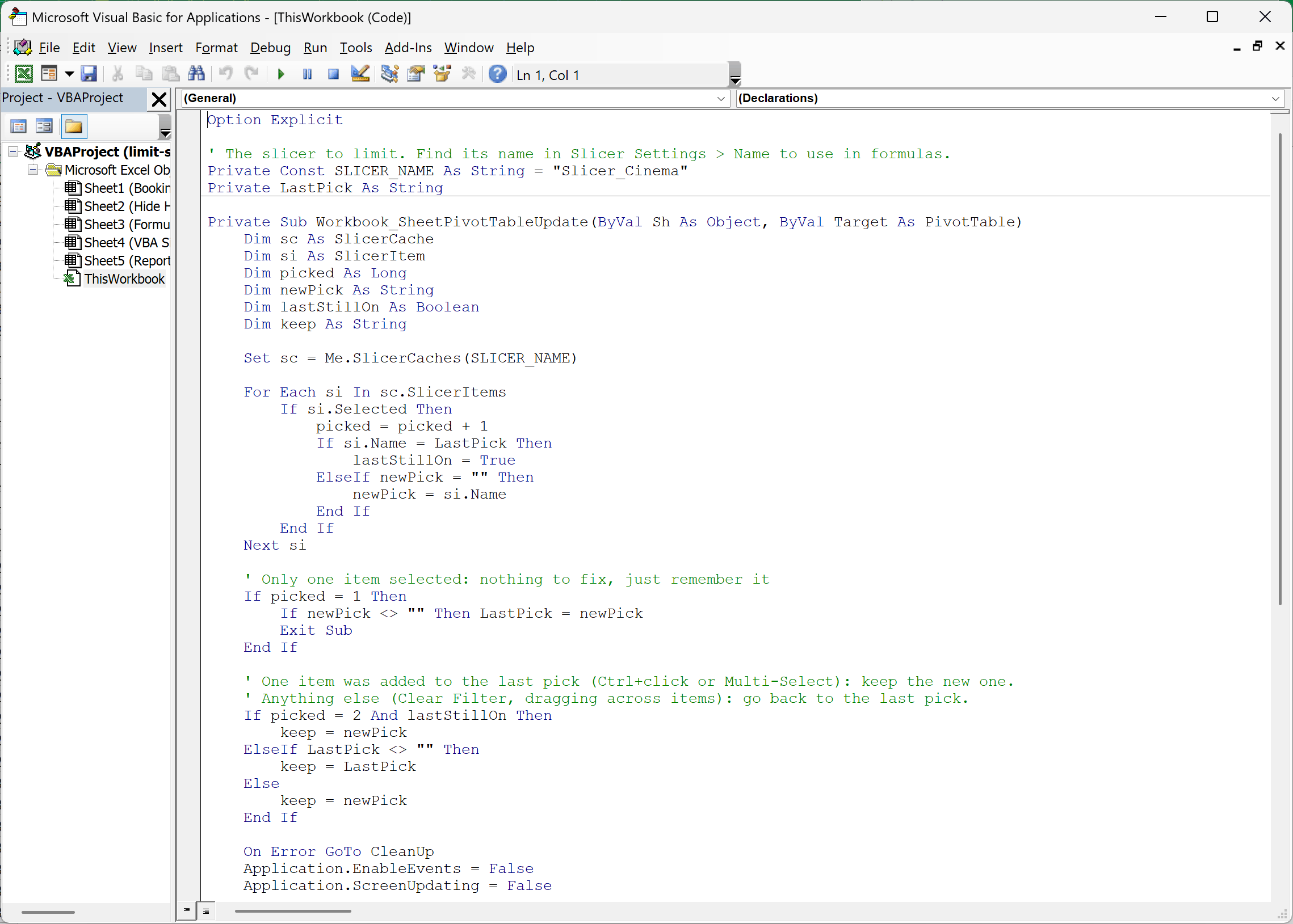
- Close the VBA editor. Then save the file as an Excel Macro-Enabled Workbook (*.xlsm), or Excel will drop the code.
Now, when you Ctrl+click Riverside while Downtown is selected, the macro turns Downtown off. Only Riverside stays selected, and the PivotTable shows Riverside’s numbers.
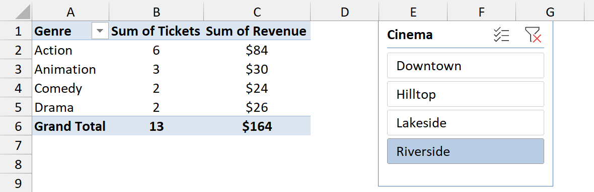
The same thing happens if you turn on Multi-Select and click a second cinema. If you click Clear Filter, the macro puts back the cinema you last picked.
How does this code work?
Excel doesn’t have an event for a slicer click. But clicking a slicer updates its PivotTable, and the Workbook_SheetPivotTableUpdate event runs every time a PivotTable updates.
The code counts the selected items and remembers the last single item in the LastPick variable.
When exactly one new item has been added to the last pick, it keeps the new item.
In every other case, such as Clear Filter selecting everything, it goes back to LastPick. Turning off EnableEvents stops the macro from running again while it changes the slicer.
Note: The macro only watches the slicer named in SLICER_NAME. Other slicers in the same workbook still allow multiple selections.
The download file for this article is an .xlsm file with this code already in it.
Since it’s a macro file downloaded from the internet, Excel blocks the macros at first. Right-click the file, choose Properties, check Unblock, and click OK before you open it.
Method #4: Using a Report Filter Instead of a Slicer
If what you really need is a filter that only accepts one choice, a PivotTable report filter does that without any code.
It’s a drop-down rather than buttons, but it’s single-select by default.
Below I have a PivotTable that shows tickets and revenue by genre for a chain of cinemas.
It has no slicer, and I want people to pick one cinema at a time.
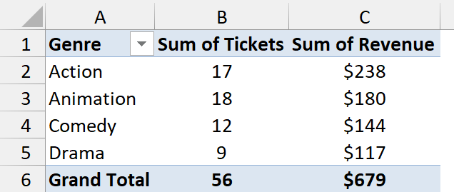
Here are the steps to add a single-select report filter:
- Click anywhere in the PivotTable, then drag Cinema into the Filters box in the PivotTable Fields pane.
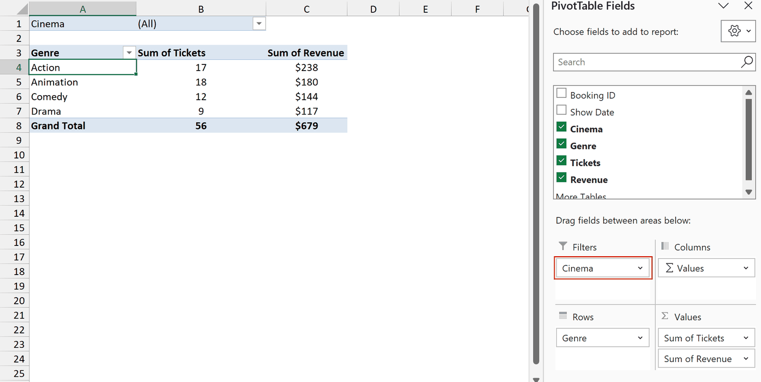
- Click the drop-down arrow in cell B1, select Downtown, and click OK. Leave Select Multiple Items unchecked.
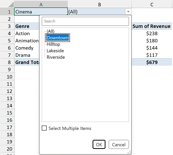
The PivotTable now shows only Downtown, and the drop-down lets people switch to one other cinema at a time.
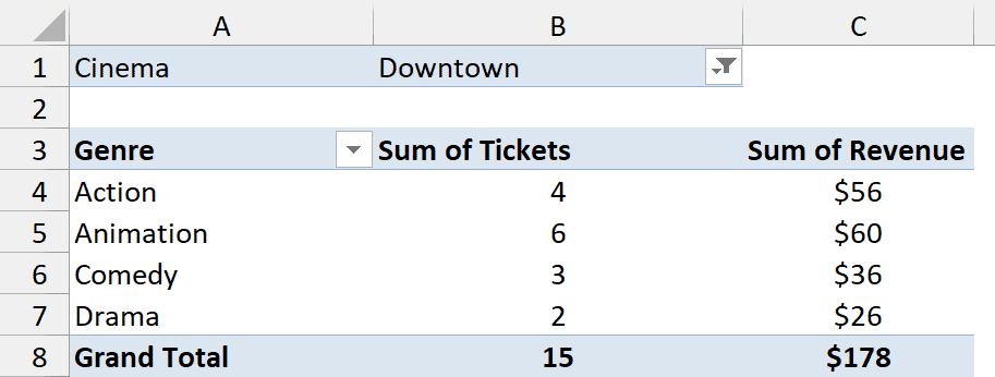
As long as Select Multiple Items stays unchecked, there’s no way to pick two cinemas.
The catch is that anyone can check that box.
I’d go with this method for a simple report where a drop-down is fine. If people expect clickable slicer buttons, use Method #3 instead.
Setting a Default Slicer Selection When the File Opens
A report often has one item people should see first, like your main location.
A Workbook_Open macro can select that item every time the file opens, no matter how it was left.
Add this code below the Method #3 code, in the same ThisWorkbook module:
Private Sub Workbook_Open()
    Const DEFAULT_ITEM As String = "Downtown"
    Dim si As SlicerItem

    Application.EnableEvents = False
    With Me.SlicerCaches(SLICER_NAME)
        .SlicerItems(DEFAULT_ITEM).Selected = True
        For Each si In .SlicerItems
            If si.Name <> DEFAULT_ITEM Then si.Selected = False
        Next si
    End With
    LastPick = DEFAULT_ITEM
    Application.EnableEvents = True
End Sub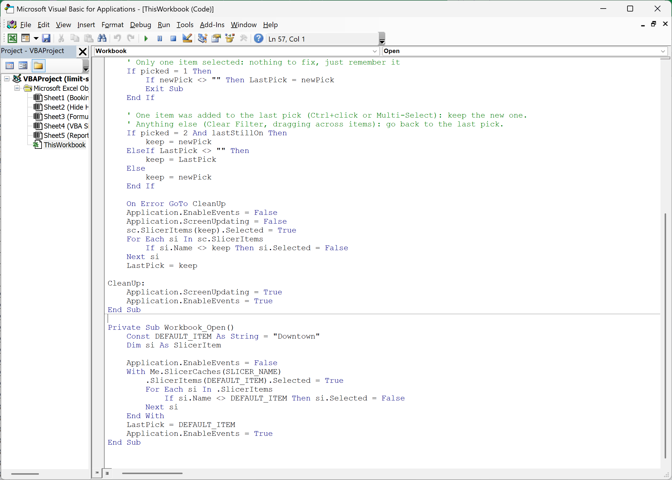
Save the file, close it, and open it again. The Cinema slicer is back on Downtown, even if someone saved it on another cinema.
The code selects Downtown first and then turns off every other item, so the slicer is never left empty along the way.
The last line tells the Method #3 macro which cinema is selected.
Note: If you’re not using the Method #3 macro, replace SLICER_NAME with your slicer’s name in quotes, like “Slicer_Cinema”, and delete the LastPick line.
Additional Notes About Limiting a Slicer to One Selection in Excel
- The steps here are for Excel on Windows. On a Mac, the VBA editor and the file-unblocking step work differently.
- Macros need a desktop version of Excel. VBA doesn’t run in Excel for the web, so Methods #1, #2, and #4 are your options there.
- Anyone can turn macros off. If someone opens the file without enabling macros, the slicer allows multiple selections again. The Method #2 warning still works in that case, so it’s a good backup.
- The macro can be slow on long slicers. It turns items off one at a time, and each change refreshes the PivotTable. For a slicer with hundreds of items, expect a short pause.
Frequently Asked Questions
Here are some common questions about single-select slicers in Excel.
Is there a setting to make a slicer single-select in Excel?
No. Excel has no option for this. Hiding the header removes the Multi-Select button, but Ctrl+click still works.
For a slicer, a macro is the only way to enforce one selection.
Why does the macro keep the wrong item after I edit the code?
Editing the code resets VBA, which clears the LastPick variable. Until you click a single item normally, the next Ctrl+click may keep the wrong one.
Does this macro work with Data Model slicers?
Not as written. For a Data Model slicer, VBA can’t loop through SlicerItems or change an item’s Selected property. You set the selection with the slicer’s VisibleSlicerItemsList property instead.
Conclusion
Excel doesn’t have a single-select slicer, so every method here is a workaround. Hiding the header makes a second selection less likely, and the formula warning makes it obvious.
When you need a hard limit, the VBA macro is the one to use.
I’d also keep the formula warning in place for anyone who opens the file with macros turned off.
I hope you found this article helpful.
Other Excel articles you may also like:
