How to Select Multiple Cells in Excel

If you want to select a bunch of cells in Excel and do something to all of them at once, dragging the mouse across them is usually the first thing you try.

And that falls apart the moment the range is bigger than your screen, or the cells you want are scattered around the sheet. But nothing to worry about.

Excel has a lot of faster ways to do this, and in this article I’ll show you 11 of them, covering mouse tricks, keyboard shortcuts and a small VBA macro.

Method #1: Using Click and Drag

This is the one everybody starts with, and for a small block of cells it’s still the quickest thing you can do.

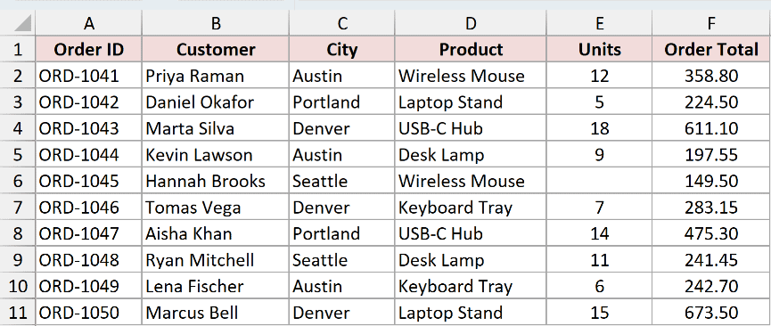
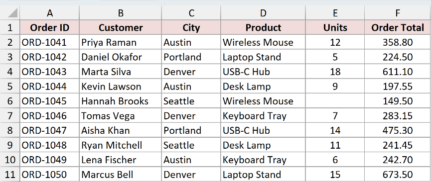
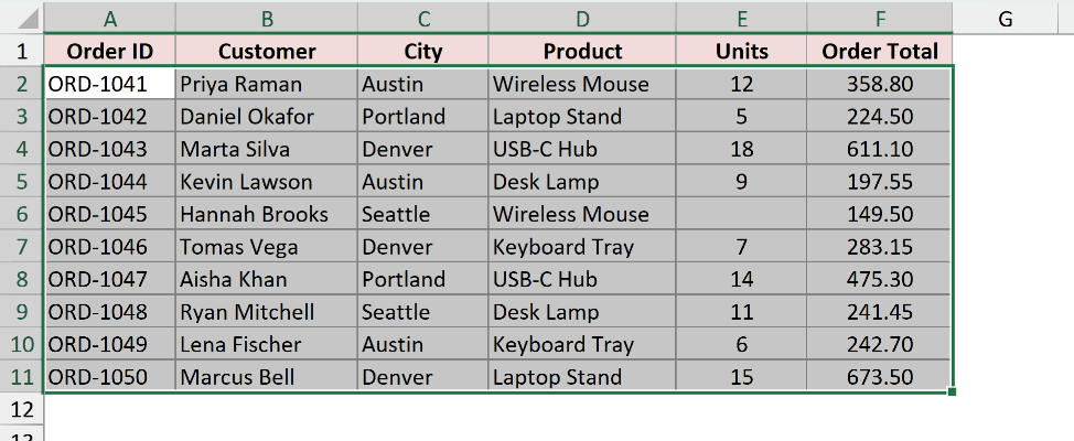
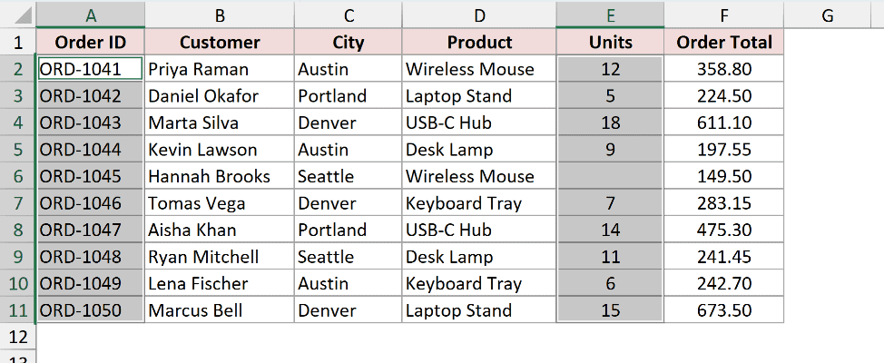
Below I have an orders dataset in the range A1:F11, with the Order ID, customer, city, product, units and order total. Let’s say I want to select the whole thing so I can format it.

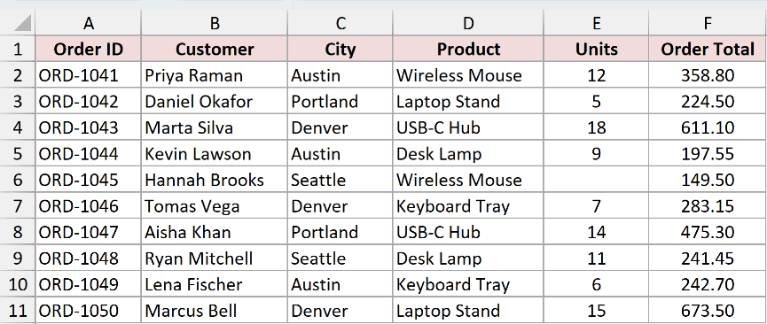
Here are the steps to select the cells by dragging:

1. Click on cell A1 and hold the left mouse button down.

2. Drag the cursor down and across to cell F11, then let go of the mouse button.

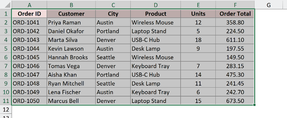
The whole range A1:F11 is now selected, and cell A1 stays white because that’s the active cell in the selection.

The catch with dragging shows up on bigger datasets. Once you hit the bottom of the visible window, Excel starts auto-scrolling, and it scrolls a lot faster than you can react. That’s when the next method saves you.

Method #2: Using the Shift Key

Here’s another way to do the exact same thing, without any dragging at all. I reach for this one more than anything else on this list.

Same orders dataset in A1:F11, and the goal is the same. I want the full block selected.

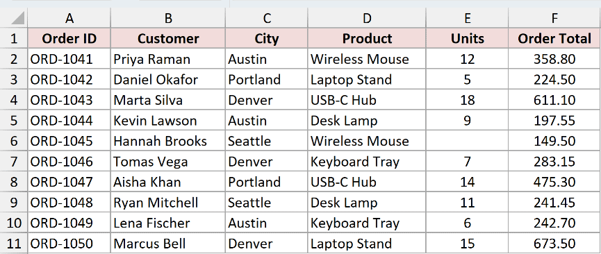
Here are the steps to select the range using the Shift key:

1. Click on cell A1.

2. Scroll down to cell F11 if you need to, hold the Shift key, and click on F11.

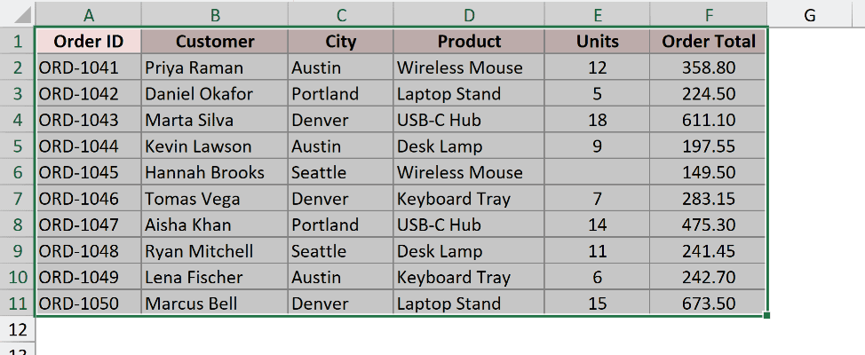
Excel selects everything between the two cells you clicked, which here is A1:F11.

Scrolling between the two clicks doesn’t break anything. Excel only cares about the first cell you clicked and the cell you Shift-clicked, so the range can be as big as you like.

You can also do this with just the keyboard. Hold Shift and tap the arrow keys, and the selection grows one cell at a time in whichever direction you press.

Note: Shift+click always extends from the active cell, which is the white one in the current selection. If you get a range you didn’t expect, check which cell is white before you click again.

Method #3: Using Ctrl+Shift+Arrow Keys

If your data runs for thousands of rows, you don’t want to scroll to the bottom just to Shift-click it. This shortcut jumps to the edge of the data and selects everything along the way.

Same dataset, and this time I want to select all the Order IDs in A2:A11.

Here are the steps:

1. Click on cell A2, the first Order ID.

2. Hold Ctrl and Shift together, then press the Down arrow key.

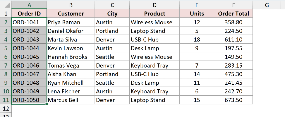
Excel selects A2:A11 in one go, stopping at the last Order ID instead of running off to row 1048576.

Try the same thing on the Units column, though, and you get a much smaller selection than you expected.

Click on E2 and press Ctrl+Shift+Down, and Excel selects E2:E5 only. It stops there because E6 is empty, and this shortcut runs until it hits a blank cell.

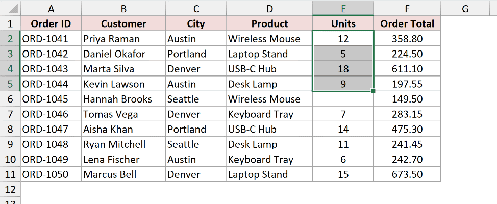
Press Ctrl+Shift+Down again and the selection jumps the gap to E2:E7. Press it a third time and you finally get E2:E11.

Note: If you want the whole used area in one shot regardless of blanks, click A2 and press Ctrl+Shift+End. That selects A2:F11 here, all the way to the last used cell on the sheet.

Method #4: Using the Ctrl Key (Non-Adjacent Cells)

Everything so far selects one solid block. When the cells you want are in different parts of the sheet, the Ctrl key is what you need.

In the orders dataset, say I want the Order IDs and the Units, but nothing in between.

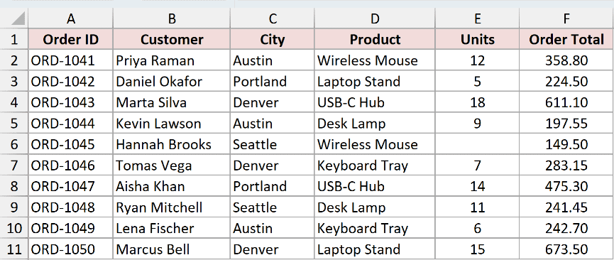
Here are the steps to select non-adjacent cells:

1. Select A2:A11 the usual way, by dragging or with Shift+click.

2. Hold the Ctrl key down and drag over E2:E11.

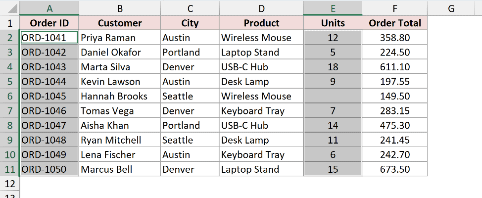
Both ranges are selected now, 20 cells across the two columns, with everything in between left alone.

Keep holding Ctrl and you can keep adding as many separate cells and ranges as you want.

There’s a lot more to this one, including doing it with the keyboard only. I’ve covered all of it in this guide on how to select non-adjacent cells in Excel.

Note: Ctrl+click also works in reverse. Ctrl+click a cell that’s already selected and Excel drops it from the selection instead of adding it again. This needs Office 2019 or a Microsoft 365 subscription, and on a Mac it’s the Cmd key.

Method #5: Using Ctrl+Space and Shift+Space

Clicking a column letter or a row number works fine, but it means taking your hand off the keyboard and aiming at a small target. These two shortcuts do it from wherever your cursor already is.

Same orders dataset, and I want the entire Units column selected.

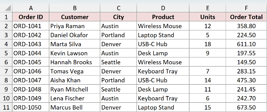
Click on any cell in column E, say E4, and press Ctrl+Space.

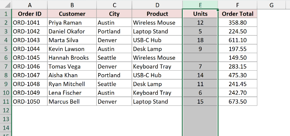
The whole of column E is selected, header and all, right down to the bottom of the worksheet.

Shift+Space is the row version. With E4 selected, press Shift+Space and Excel selects the whole of row 4, which is the ORD-1043 order.

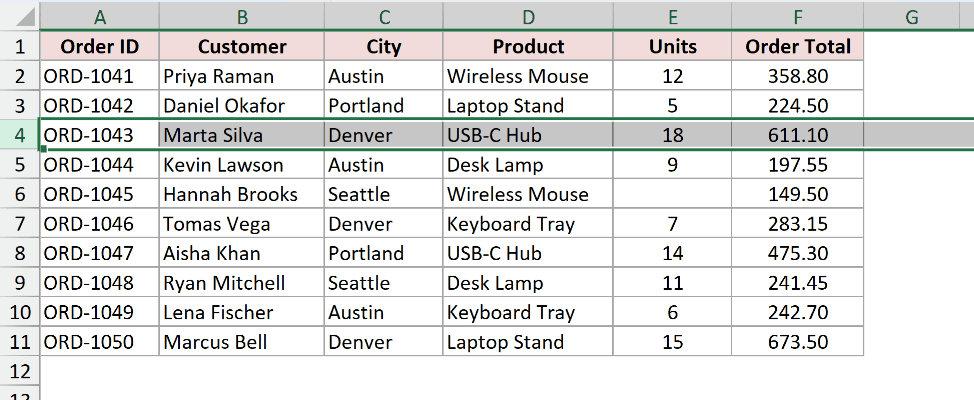
Both shortcuts stack with Ctrl. Select the whole of column E, then hold Ctrl and press Ctrl+Space on a cell in column A, and you get two entire columns.

If rows are what you’re really after, I’ve written a separate guide on how to select multiple rows in Excel.

Method #6: Using the Ctrl+A Shortcut

When you want the whole dataset and nothing else, this is a single keystroke.

Here’s the orders dataset again, sitting in A1:F11 with empty cells all around it.

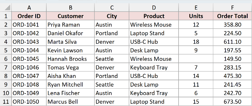
Click on any cell inside the data, say C5, and press Ctrl+A.

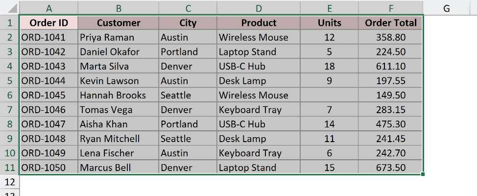
Excel selects A1:F11, which is the whole block including the header row.

Press Ctrl+A a second time and the selection expands to every cell in the worksheet. Ctrl+Shift+Space gets you there in one go, and the Select All button, that little triangle above row 1 and left of column A, does it with a single click.

Note: Ctrl+A stops at a completely empty row or column, not at a single empty cell. The blank in E6 doesn’t split this dataset, but an entirely blank row 6 would, and you’d only get A1:F5.

Method #7: Using the Name Box

Here’s the one for when you already know the address of what you want. No scrolling, no dragging, and it doesn’t care how big the range is.

The Name Box is the small box to the left of the formula bar, the one showing the address of the current cell.

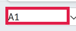
Here are the steps to select a range using the Name Box:

1. Click inside the Name Box and type A2:F11.

2. Press the Enter key.

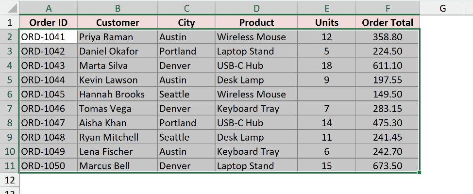
Excel jumps straight to that range and selects it, all ten rows across all six columns.

Non-adjacent ranges work here too. Type A2:A11,E2:E11 into the Name Box and press Enter, and you get the Order IDs and the Units selected together.

This is also the fastest way to select something like A1:A50000. Typing the address takes two seconds, and dragging there takes a lot longer than that.

Method #8: Using the Go To Dialog Box

The Go To dialog does the same job as the Name Box, with one difference that matters if you keep coming back to the same ranges. It remembers them.

Same orders dataset, and I want the Order IDs and Units selected again.

Here are the steps:

1. Press Ctrl + G to open the Go To dialog box. The F5 key does the same thing.

2. Type A2:A11,E2:E11 into the Reference box and click OK.

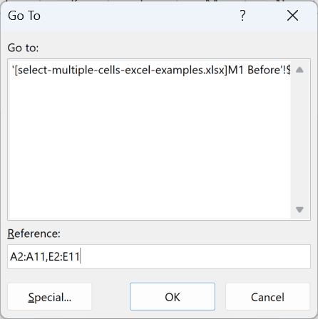
Both ranges get selected, exactly like the Name Box version.

Open Go To again and you’ll see that reference sitting in the list at the top of the dialog. Double-click it and you’re back on that selection, which is handy when you’re checking the same block over and over.

Method #9: Using Go To Special

Every method up to here selects cells based on where they sit. This one selects them based on what’s inside them, and that makes it the most useful trick on the whole list.

In the orders dataset there’s one missing value in the Units column, and on a real sheet with a few thousand rows you’d never spot it by eye.

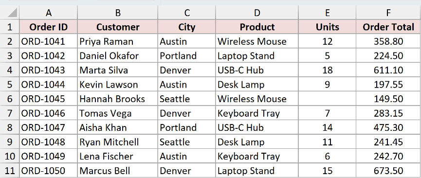
Here are the steps to select the blank cells:

1. Select the range you want to search, which is E2:E11 here.

2. Press Ctrl + G, then click the Special button at the bottom of the dialog. You can also get there from the Home tab, then Find & Select, then Go To Special.

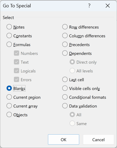
3. Select the Blanks option and click OK.

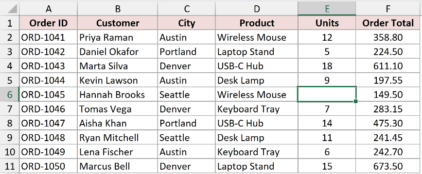
Excel selects cell E6, the only empty cell in that range.

Blanks is just one of the options. Formulas selects every cell holding a formula, Constants selects every cell where somebody typed a value, and Visible cells only skips anything hidden by a filter.

That last one has a few quirks of its own, and I’ve covered them in this guide on how to select visible cells only in Excel.

Note: Go To Special works inside your selection if you have more than one cell selected, and across the entire worksheet if you only have one cell selected. Select the range first, or you’ll get every blank cell on the sheet.

Method #10: Using Extend Selection Mode (F8)

If you’d rather not hold keys down while you navigate, Excel has a mode that does the holding for you.

Here’s the orders dataset one more time, and the goal is to select A2:F11 without touching the mouse.

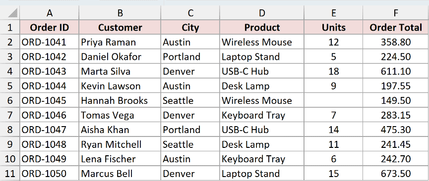
Here are the steps:

1. Click on cell A2 and press the F8 key. Look at the status bar at the bottom left and you’ll see Extend Selection.

2. Use the arrow keys to move down to row 11 and across to column F. The selection grows as you go, with no keys held.

3. Press F8 again, or press Esc, to turn the mode off.

Press Shift + F8 instead and the status bar reads Add or Remove Selection, which lets you click extra ranges into the selection without holding Ctrl. Press Shift + F8 again or Esc to come back out.

Note: If your selection keeps growing every time you click somewhere, you’re stuck in one of these modes, usually from hitting F8 by accident. Check the status bar and press Esc to get out.

Method #11: Using a VBA Macro

If you find yourself rebuilding the same awkward selection every morning, hand it to a macro instead.

Same orders dataset, and I want the Order IDs and the Units selected in one click.

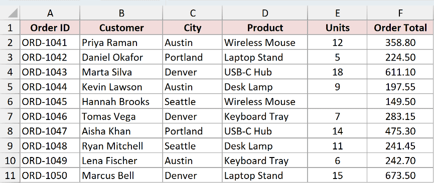
Here is the VBA code:

Sub SelectOrderIDsAndUnits()
    Range("A2:A11,E2:E11").Select
End Sub

Sub SelectOrderIDsAndUnits()
    Range("A2:A11,E2:E11").Select
End Sub

Here are the steps to use this macro:

1. Press Alt + F11 to open the VBA Editor.
2. Go to Insert, then Module, to add a new module.
3. Paste the code above into the module.
4. Press F5 to run it.

The comma inside the range string is what makes this a multi-area selection, and you can add as many comma-separated ranges as you need.

When the addresses aren’t fixed, Union does the same job with separate Range objects, like Union(Range(“A2:A11”), Range(“E2:E11”)).Select. There’s a lot more you can do here, and I’ve covered the variations in this guide on selecting a range in Excel using VBA.

Note: A workbook with a macro in it has to be saved as .xlsm. Save it as a normal .xlsx and Excel throws the code away without much of a warning.

Additional Notes About Selecting Multiple Cells in Excel

• The status bar is your check. Select anything and the bottom right shows Count, and for numbers it also shows Sum and Average. Selecting E2:E11 in this dataset gives Count 9 and Sum 97, and a Count of 9 instead of 10 is the fastest way to spot that missing value in E6.
• The white cell in a selection matters. That’s the active cell, and typing only fills that one. Type your value and press Ctrl + Enter instead of Enter and Excel fills every selected cell at once.
• Don’t select entire columns for conditional formatting or formulas. Applying a rule to E:E means Excel is watching a million cells instead of ten. Select the actual used range and your file stays fast.
• Selecting every Nth cell isn’t a plain selection job. Ctrl+click gets old very quickly past a few rows, so if that’s what you’re after, take a look at how to select every other cell in Excel.
• On a Mac, not every Ctrl turns into Command. Ctrl+Space for a column and Shift+Space for a row are exactly the same on both platforms. Ctrl+A becomes Cmd+A, and the Name Box and Go To dialog work identically.

Frequently Asked Questions

Why do I get “That command cannot be used on multiple selections” when I copy?

Excel can only copy a non-adjacent selection when the pieces line up into a rectangle once you squeeze out the gap.

Same rows across different columns is fine, so A2:A11 plus E2:E11 copies without complaint. Something like B2:B5 plus E7:E11 doesn’t, because the rows and the columns are both different.

Copy the pieces one at a time, or move the columns next to each other first.

How do I deselect one cell without losing the whole selection?

Hold Ctrl and click the cell you want to drop, and Excel removes it from the selection. Hold Ctrl and drag to remove a whole block. Ctrl+click it again and it comes back.

Why does my selection keep growing when I click somewhere else?

You’re in Extend Selection or Add or Remove Selection mode, which happens when F8 or Shift + F8 gets pressed by accident. Look at the bottom left of the status bar, and press Esc to get back to normal.

Can I select the same cells on several sheets at once?

Yes. Ctrl+click or Shift+click the sheet tabs first to group them, then make your selection. Whatever you type or format applies to that cell on every grouped sheet.

Right-click a tab and choose Ungroup Sheets when you’re done. Forgetting to is an easy way to wreck three sheets at once.

Why does typing only fill one cell when I have a whole range selected?

Because Excel puts what you type into the active cell only, which is the white one. Press Ctrl + Enter instead of Enter and the same value lands in every cell in the selection.

Conclusion

Selecting cells in Excel gets a lot less annoying once you stop dragging. For everyday work, Shift+click is the one to build the habit around, and Ctrl+Shift+Arrow takes over the moment your data is bigger than the screen.

Keep the Name Box in mind for ranges you can name off the top of your head, and Go To Special for the days when you need the blanks rather than the block.

Between those four, you’ll almost never reach for the mouse again.

Other Excel articles you may also like:

• How to Select Every Other Row (Alternate Row) in Excel?
• How to Select Alternate Columns in Excel (or every Nth Column)
• How to Select Rows with Specific Text in Excel
• How to Select Multiple Items from a Drop Down in Excel?
• Select Row (or Rows) in Excel (Shortcut)
• How to Delete Multiple Rows in Excel?
• How to Apply Formula to Entire Column in Excel?
• Arrow Keys Not Working in Excel (Not Moving Between Cells)
• Excel Table vs. Excel Range – What’s the Difference?