
Tally marks give you a quick visual count of votes, survey answers, attendance, or anything else you record repeatedly.
Excel has no dedicated tally button. However, a couple of formulas are all you need to tally in Excel.
They count a raw list of responses and turn those totals into a useful tally sheet.
I’ll show you how to draw plain marks, group them in fives, and build a complete sorted tally sheet with one Microsoft 365 formula.
Method #1: Using COUNTIF and REPT
This method starts with the raw responses instead of a count someone has already typed. COUNTIF calculates each total, and REPT draws one mark per vote.
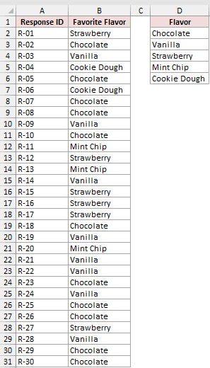
Below I have a dataset with 30 survey responses in A1:B31 and a typed flavor list in D2:D6. I want to count each flavor first.
Enter this formula in cell E2:
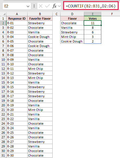
=COUNTIF(B2:B31,D2:D6)
How does this formula work?
COUNTIF checks B2:B31 against each flavor in D2:D6 and returns all five vote counts.
The formula spills down the column automatically. It returns 11 Chocolate, 8 Vanilla, 6 Strawberry, 3 Mint Chip, and 2 Cookie Dough votes.
Next, enter this formula in cell F2 to draw one pipe character for every vote:
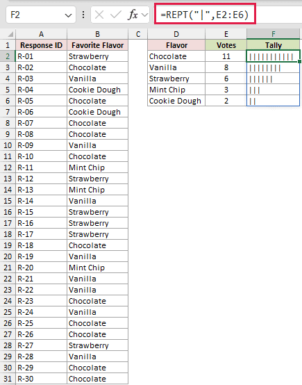
=REPT("|",E2:E6)
How does this formula work?
REPT repeats the pipe character for each vote total in E2:E6. The formula spills down the column automatically.
Chocolate has 11 votes, so its result contains 11 marks. You now have the raw responses, vote totals, and plain tally marks in one sheet.
Note: The spilling formulas in this article need Microsoft 365 or Excel 2021. On Excel 2019 or earlier, enter =COUNTIF($B$2:$B$31,D2) in E2 and =REPT("|",E2) in F2, then fill both down to row 6. The same fill-down approach works for Method #2.
Method #2: Using REPT With INT and MOD
Here’s another way to draw the marks. This is the method I recommend for most people because groups of five are much easier to scan.
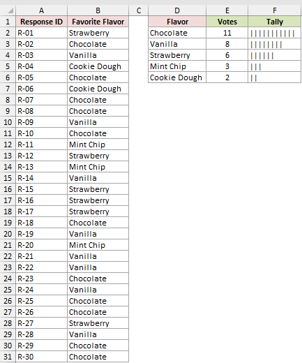
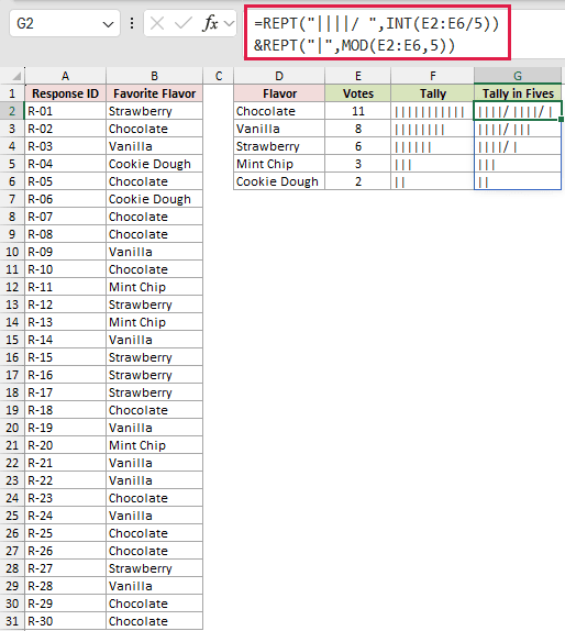
Below I have the same 30 survey responses, the flavor list, and the vote totals in E2:E6. I want to display those totals in five-mark groups.
Enter this formula in cell G2. The formula spills down the column automatically.
=REPT("||||/ ",INT(E2:E6/5))&REPT("|",MOD(E2:E6,5))
How does this formula work?
INT(E2:E6/5) returns the number of complete five-vote groups for each flavor. For 11 Chocolate votes, it returns 2.
The first REPT draws each complete group as four pipes and a slash. The trailing space keeps adjacent groups from running together.
MOD(E2:E6,5) returns the votes left after each complete group. The second REPT draws those remaining marks, and the ampersand joins both parts.
The finished results are ||||/ ||||/ |, ||||/ |||, ||||/ |, |||, and || for the five flavors.
Note: REPT keeps every mark on one line. For large counts, widen the column or use this grouped-in-fives style to keep the tally readable.
Method #3: Using One Spilled Formula (Microsoft 365)
If you have Microsoft 365, one formula can create the flavor list, count every response, draw grouped marks, and sort the finished tally sheet.
Below I have the 30 survey responses in A1:B31 and an empty area beginning in D2. I want the complete tally table to spill into that area.
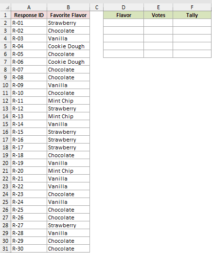
Enter this formula in cell D2:
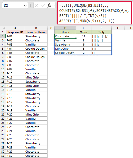
=LET(f,UNIQUE(B2:B31),v,COUNTIF(B2:B31,f),SORT(HSTACK(f,v,REPT("||||/ ",INT(v/5))&REPT("|",MOD(v,5))),2,-1))
How does this formula work?
LET assigns the unique flavors to f and their vote totals to v. Those short names keep the rest of the formula manageable.
UNIQUE extracts each flavor once from B2:B31. COUNTIF then counts the responses for every flavor in that spilled array.
The two REPT parts draw complete five-mark groups and leftover marks. INT calculates the complete groups, while MOD calculates the remainder.
HSTACK places the flavors, vote totals, and tally marks in three columns. SORT orders the combined array by its second column, from highest to lowest.
The formula spills the five completed rows automatically, with Chocolate first at 11 votes and Cookie Dough last at 2 votes.
The tally updates when a response changes inside B2:B31. A fixed range will not include new responses entered below row 31.
Extend the references when you add more rows. You can also convert the source to an Excel Table and use an expanding structured reference.
How to Make a Tally Sheet in Excel
Keep the raw data on one side and the compact Flavor, Votes, and Tally table together. Adjust the tally column width before checking the sheet in Print Preview.
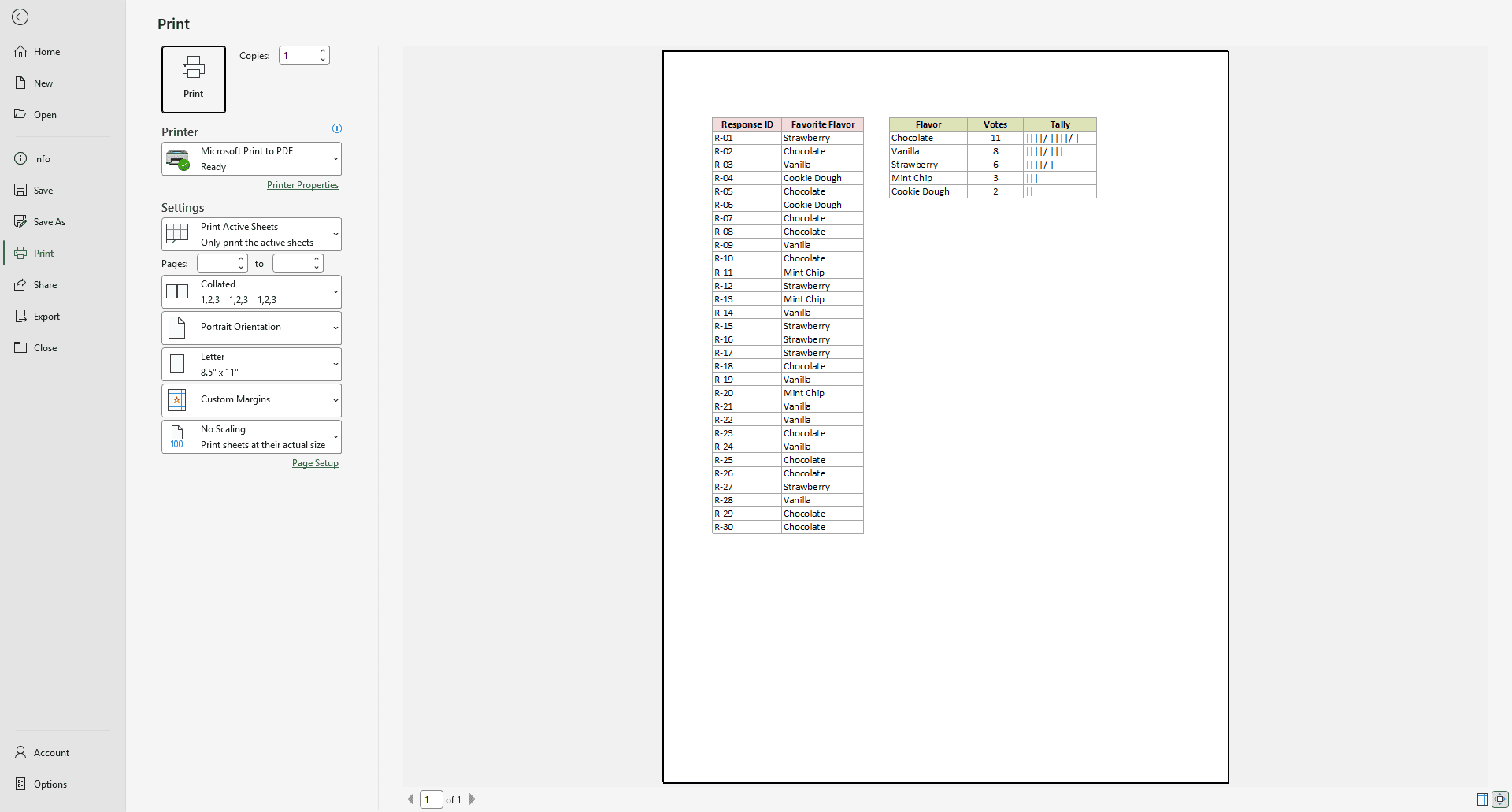
Grouped marks take less horizontal space than a long row of single pipes, so Method #2 is usually the best layout for printing.
Additional Notes About Making Tally Marks in Excel
- A regular or monospaced font can display the pipe marks. The spacing will look different, so choose the font that makes your tally easiest to read.
- The Tally column contains text, not numbers. Sum the Votes column when you need a total.
- Formula-based marks update when the source responses change. You do not need to redraw them manually.
- Left alignment keeps the marks reading naturally across the cell. Center alignment can work better on a compact printed tally sheet.
Frequently Asked Questions
Is There a Tally Mark Symbol in Excel?
Unicode includes TALLY MARK ONE and TALLY MARK FIVE. Their codes are UNICHAR(119671) and UNICHAR(119672).
In Excel for Windows, both appeared as empty boxes in Aptos, Calibri, Segoe UI Symbol, Segoe UI Emoji, and Cambria Math during testing.
The pipe-and-slash REPT formulas are the safer choice because those ordinary characters render reliably.
Can I Tally Checkmarks or X Marks Instead?
Yes. Replace the pipe inside REPT with the character you want, such as =REPT("X",E2). Excel will repeat that character once for every vote.
How Do I Count Tally Marks Back Into Numbers?
Use =LEN(F2) for the plain one-mark-per-vote tally. LEN counts the characters in F2, so 11 pipe characters return 11.
This does not work for the grouped tally because its slashes and spaces are also characters. Use the Votes column for grouped results.
Conclusion
In this article, I showed you how to turn a raw list of responses into tally marks using COUNTIF and REPT.
I also showed you how to group those marks in fives and how to build the whole tally sheet with one spilled formula.
I hope you found this article helpful.
Other Excel articles you may also like:
