Generate All Possible Combinations from Two Lists

In Excel, you may sometimes want to generate all possible combinations from two lists, for instance, to display all product variations.

I will show you how to accomplish this in this tutorial using Power Query, formulas, and VBA.

Method #1: Power Query to Generate All Possible Combinations from Two Lists

Suppose you have a list of six car types and another list of five colors.

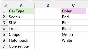
You want to combine every car type on the first list with every color on the second.

Note: By pairing each car type with every color, we expect to get 30 possible combinations (6 × 5).

Here’s how to do it using Power Query:

Step #1: Convert the Lists to Excel Tables

1. Select a cell in the first list and press CTRL + T.

The above step opens the Create Dialog box with the range reference of the list filled in and the ‘My table has headers’ checkbox selected.

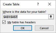
2. Click OK on the Create Table dialog box.

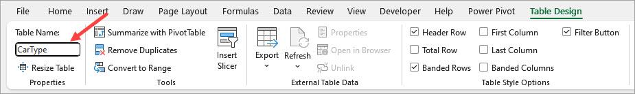
The above step creates a table and gives it the default name Table1. 

You can give the table a meaningful name by renaming it in the Table Name box, on the Properties group of the Table Design tab. In this example, I renamed it ‘CarType.’ 

3. Repeat steps 1 and 2 for the second list.

The above step creates a table and gives it the default name Table2. Rename the table to a meaningful name. In this example, I have renamed it ‘Color.’

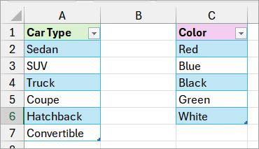
Finally, you have two Excel tables as shown below.

Step #2: Load the Table Data Onto Power Query

1. Select any cell in the ‘CarType’ table.
2. Open the Data tab and click the From Table/Range command button on the Get & Transform Data group.

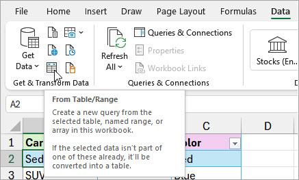
The above step opens Power Query and loads the table data onto the Power Query Editor.

3. On the Home tab of the Power Query Editor, click the lower part of the Close & Load button on the Close group, and select the Close & Load To option.

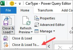
The above step opens the Import Data dialog box.

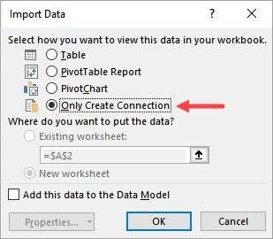
4. On the Import Data dialog box, select the ‘Only Create a Connection’ option and click OK.

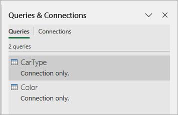
5. Do steps 1 to 4 for the ‘Color’ table.

These steps create two queries listed on the Queries & Connections pane on the right side of the Excel window.

Step #3: Create a New Query Joining the Two Queries 

1. Press ALT + F12 to open a new Power Query Editor window.
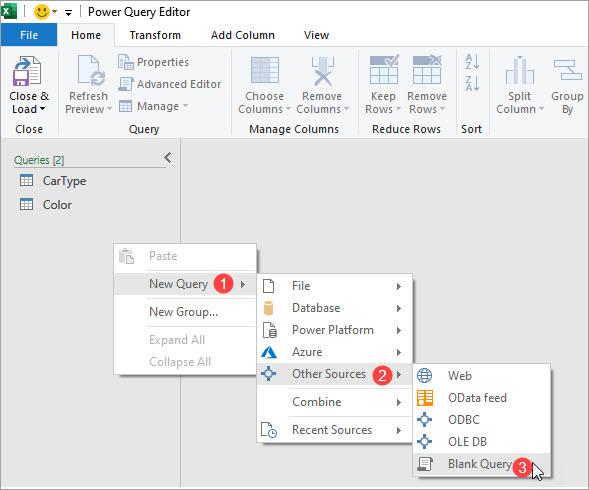
2. On the Power Query Editor, right-click a blank area on the navigation pane on the left, hover over the New Query option on the shortcut menu, hover over the Other Sources option on the first submenu, and select Blank Query on the final submenu.

The above step opens a blank Query1 query on the navigation pane on the left side of the Power Query Editor.

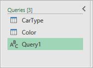
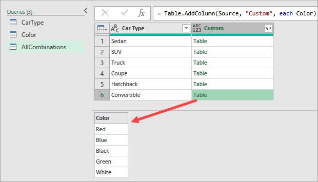
3. Double-click Query1 and give it a meaningful name. I have named it ‘AllCombinations.’
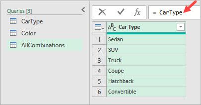
4. In the navigation pane on the left, select the ‘AllCombinations’ query. Then, in the formula bar, ‘type = CarType.’ This will load all the data from the ‘CarType’ query into the Power Query Editor.

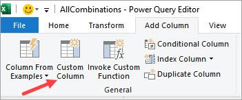
5. Open the Add Column tab and click the Custom Column command button on the General group.

The above step opens the Custom Column feature.

6. On the ‘Custom column formula’ box on the Custom Column feature, enter the formula ‘= Color’ and click OK. 

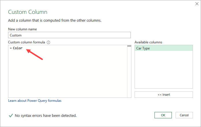
The above step inserts the ‘Color’ table data in each cell of the new custom column.

7. Click the expand button in the header of the new column, uncheck the ‘Use original column name as prefix’ checkbox, and click OK.

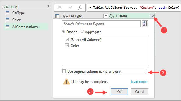
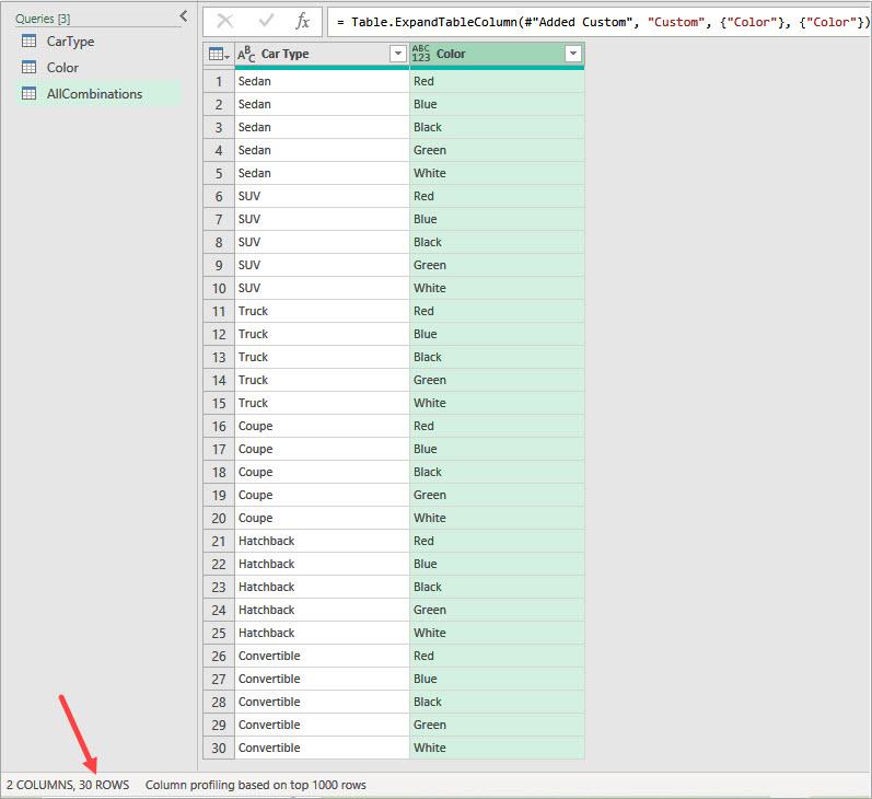
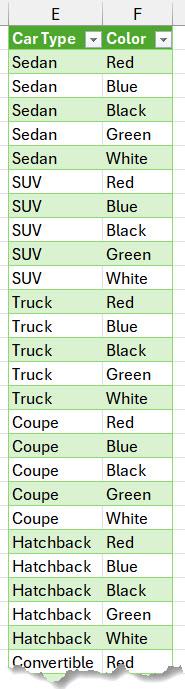
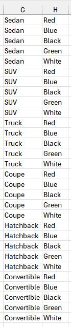
The above step generates 30 records, representing all possible combinations from the two tables.

Step #4: Load the Query Data Onto Excel Worksheet

1. On the Home tab of the Power Query Editor, click the lower part of the Close & Load command button on the Close group, and select the Close & Load To option.

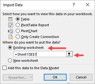
The above step opens the Import Data dialog box.

2. On the Import Data dialog box, select where to put the data and click OK. In this example, I have chosen the ‘Existing worksheet’ option, starting at cell E1. 

The above step puts the data in the worksheet you chose. The data represents all 30 possible combinations from the ‘Car Type’ and ‘Color’ lists.

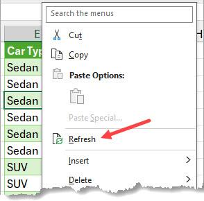
Note: If you modify the initial two tables, such as adding new car types to the first table, right-click any cell in the results table and select Refresh. This will update the results table accordingly.

Also read: Combine Two Columns in Excel (with Space/Comma)

Method #2: Formula to Generate All Possible Combinations from Two Lists

You can use a formula combining TOCOL and TRANSPOSE functions to create all possible combinations from two lists.

Suppose you have the below lists of six car types and five colors.

You want to combine every car type on the first list with every color on the second list. 

Note: By pairing each car type with every color, we should get 30 possible combinations (6 × 5).

Here’s how to do it using a formula:

1. Select the cell where you want to enter the formula. In this example, I have chosen cell E1.
2. Enter the following formula and press Enter.

=TOCOL(A2:A7&"|"&TRANSPOSE(C2:C6))

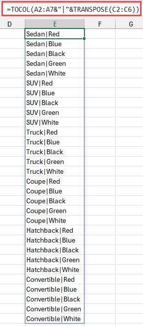
Note: The formula produces all possible combinations from the two lists in but in one column. To split the results into separate columns, use the TEXTSPLIT function as shown below.

3. Enter the following formula in cell G1:

=TEXTSPLIT(E1,"|") 

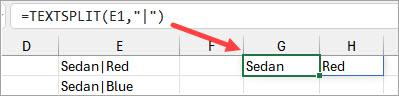
4. Drag the fill handle in cell G1 to the last row of data in column E.

Explanation of the Formula

=TOCOL(A2:A7&”|”&TRANSPOSE(C2:C6))

This formula generates all possible pairwise combinations between the two lists, separated by a pipe ( | ), and outputs them in a single vertical column.

Here’s how it does it:

• A2:A7 – This is a vertical list of 6 car types.
• C2:C6 – This is a vertical list of 5 colors.
• TRANSPOSE(C2:C6) – Converts the vertical list of 5 colors into a horizontal row of 5 columns.
• A2:A7&”|”&TRANSPOSE(C2:C6) – Performs a pairwise concatenation. Since A2:A7 is vertical (6 rows) and TRANSPOSE(C2:C6) is horizontal (5 columns), Excel broadcasts the operation, creating a 6×5 grid where each item from A2:A7 is combined with every item from C2:C6, separated by a pipe ( | ).
• TOCOL(…) – Converts the resulting 6×5 array into a single-column array.

Method #3 – Creating a LAMBDA to Generate Combinations

Another way you can use a formula to create all possible combinations from two tables is to define a LAMBDA function in Excel and use it in a formula.

Suppose you have the two tables below: ‘CarType’ and ‘Color.’

You want to generate all possible combinations from the two tables.

Here’s how to do it using a LAMBDA function:

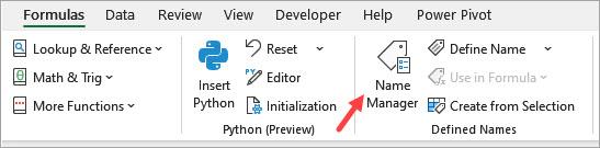
1. Open the Formula tab and click the Name Manager command button on the Defined Names group.

The above step opens the Name Manager feature.

2. Click the New command button on the Name Manager feature.

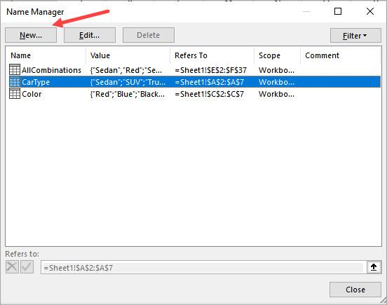
The above step opens the New Name feature.

3. Do the following on the New Name feature:

1. Enter the Name COMBINE on the Name box.
2. Copy and paste the below formula on the ‘Refers to’ box:

=LAMBDA(Table1,Table2, 
LET(LenX,ROWS(Table1), 
LenY,ROWS(Table2), 
Seq,SEQUENCE(LenX*LenY,,0), Array1,XLOOKUP(INT((Seq)/LenY)+1,SEQUENCE(LenX),Table1,””), Array2,XLOOKUP(MOD(Seq,LenY),SEQUENCE(LenY,,0),Table2,””), HSTACK(Array1, Array2)))

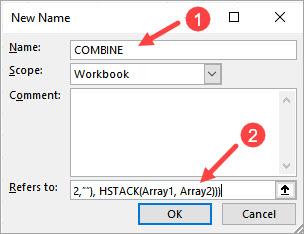
4. Click OK on the New Name feature.
5. Close the Name Manager feature.
6. Select a cell on the worksheet containing the two tables and enter the formula below.

=COMBINE(CarType,Color)

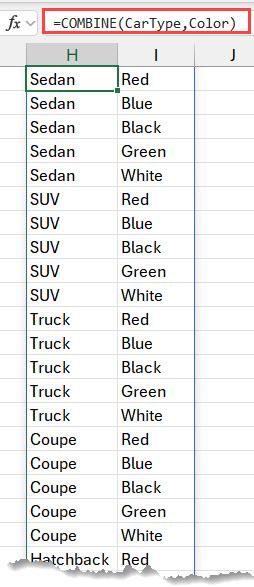
The formula returns 30 records, all possible combinations from the two tables.

Explanation of the LAMBDA Function

This Excel LAMBDA function generates all possible pairwise combinations of values from two tables (Table1 and Table2 ) using  LET to define intermediate values:

1. LenX, LenY – This calculates the number of rows in Table1 and Table2.
2. Seq – This creates a sequence from 0 to (LenX * LenY – 1) to serve as an index for pairing.
3. Array1 –  Uses  XLOOKUP to extract values from Table1, repeating each value LenY times.
4. Array2 – Uses XLOOKUP to extract values from Table2, cycling through them.
5. HSTACK – Combines Array1 and Array2 horizontally, creating a two-column array with all possible combinations.

Method #4: Using VBA User-Defined Function to Generate All Possible Combinations from Two Lists

You can create a User-Defined Function (UDF) in VBA and use it in a formula to generate all possible combinations from two lists.

Suppose you have the following lists of six car types and five colors.

Note: The first list contains six car types, and the second list has five colors. By pairing each car type with every color, we expect to get a total of 30 possible combinations (6 × 5).

You want to combine every car type on the first list with every color on the second list.

Here’s how to do it using a UDF:

1. Copy the code below and paste it into a standard VBA module.

Option Explicit
Function COMBINATIONS(rng1 As Range, rng2 As Range) As Variant
Dim i As Integer, j As Integer
Dim outputRow As Integer
Dim result() As Variant
Dim totalRows As Integer
totalRows = rng1.Rows.Count * rng2.Rows.Count
ReDim result(1 To totalRows, 1 To 2)
outputRow = 1
For i = 1 To rng1.Rows.Count
    For j = 1 To rng2.Rows.Count
        result(outputRow, 1) = rng1.Cells(i, 1).Value
        result(outputRow, 2) = rng2.Cells(j, 1).Value
        outputRow = outputRow + 1
    Next j
Next i
COMBINATIONS = result
End Function

Note: Save the workbook as a Macro-Enabled Workbook (*.xlsm) to retain the code.

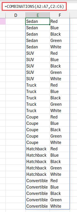
2. Enter the below formula in a cell.

=COMBINATIONS(A2:A7,C2:C6)

Explanation of the Code

The COMBINATIONS function generates all possible combinations from two lists using the steps below.

• It calculates the total number of combinations – totalRows = rng1.Rows.Count * rng2.Rows.Count
• It resizes the array ‘result’ to store the output.
• It iterates through the first list (outer loop) and the second list (inner loop), storing every combination in the ‘result’ array.
• The function outputs the ‘result’ array as a 2D array.

I have shown you how to generate all possible combinations from two lists using Power Query, formulas, and VBA. I hope you found the tutorial helpful.

Other Excel articles you may also like:

• How to Separate Names in Excel
• How to Generate Random Letters in Excel?
• How to Generate Random Names in Excel
• How to Group Duplicates in Excel
• Switch First and Last Name with Comma in Excel (Reverse Names)
• How to Flip Data in Excel (Columns, Rows, Tables)?