
Excel’s IFNA function returns a fallback value when a calculation produces #N/A. It leaves other error types unchanged.
It is useful with VLOOKUP or HLOOKUP when a missing match is expected. You can show a message while keeping unrelated calculation errors visible.
In this article, I’ll show you how to replace missing lookup results with messages or zeros, and understand when IFNA differs from IFERROR.
IFNA Function Syntax in Excel
The IFNA function checks a formula and, if it returns the #N/A error, gives you back a value of your choosing.
=IFNA(value, value_if_na)
- value – the formula or expression you want to check for the #N/A error. This is usually a lookup like VLOOKUP or MATCH.
- value_if_na – the value to return when
valueevaluates to #N/A. This can be text, a number, a blank string, or another formula.
If value does not return #N/A, IFNA simply hands back the original result.
When to Use IFNA Function
- Replace the #N/A error from VLOOKUP, HLOOKUP, or LOOKUP with a readable message like “Not Found”.
- Return 0 (or a blank) so missing lookups don’t break a SUM, AVERAGE, or other calculation downstream.
- Clean up a dashboard or report so stakeholders don’t see raw error values.
- Catch only #N/A while letting other errors (like #DIV/0! or #REF!) stay visible, so you don’t accidentally hide a real problem.
Example 1: Replace VLOOKUP #N/A With a Message
Let’s start with the most common use of IFNA, cleaning up a VLOOKUP.
Below is a small price list in columns A and B, with a set of product codes to look up in column D.
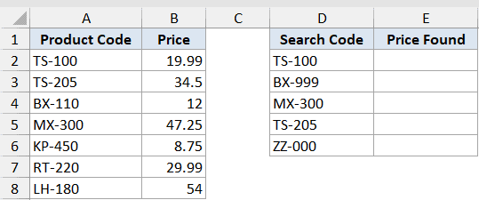
I want to pull the price for each search code in column D, and show “Not Found” whenever a code isn’t in the price list.
Here is the formula:
=IFNA(VLOOKUP(D2:D6, A2:B8, 2, FALSE), "Not Found")
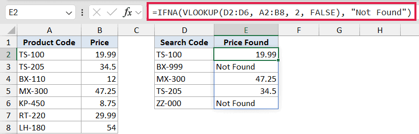
The VLOOKUP looks up each code from D2:D6 in the price table and returns the matching price. When a code like BX-999 or ZZ-000 isn’t found, VLOOKUP would normally throw #N/A. IFNA catches that and returns “Not Found” instead.
Notice that I fed VLOOKUP the whole range D2:D6 in one go. In Excel 365 the formula spills down the column automatically, so I only typed it once in cell E2.
> In Excel 365, XLOOKUP has this built in. =XLOOKUP(D2:D6, A2:A8, B2:B8, "Not Found") does the same job, with the fallback value as its fourth argument, so you don’t need to wrap it in IFNA at all. IFNA + VLOOKUP is still worth knowing for older versions of Excel and for the many sheets that already use VLOOKUP.
Example 2: Use IFNA With HLOOKUP
IFNA works with any lookup that can return #N/A, including horizontal lookups.
Below is a row of monthly targets laid out across columns, with a lookup month entered in cell B4.
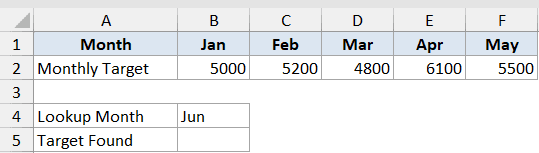
I want to pull the target for the month in B4, and show “Not tracked” if that month isn’t in the table.
Here is the formula:
=IFNA(HLOOKUP(B4, A1:F2, 2, FALSE), "Not tracked")
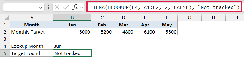
HLOOKUP scans the header row of A1:F2 for the month in B4 and returns the value from the second row. Since “Jun” isn’t in the table, HLOOKUP returns #N/A, and IFNA swaps it for “Not tracked”.
The logic is identical to the VLOOKUP version. IFNA doesn’t care which lookup function sits inside it. It only reacts to the #N/A error.
Example 3: IFNA With INDEX/MATCH
INDEX/MATCH is a flexible alternative to VLOOKUP, and it returns #N/A the same way when there’s no match.
Below is an employee list with names in column A and departments in column B, plus a set of names to look up in column D.
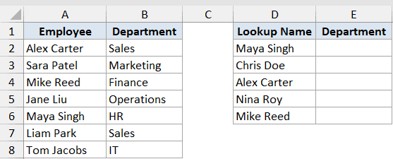
I want to find the department for each name in column D, and show “No match” for any name that isn’t on the list.
Here is the formula:
=IFNA(INDEX(B2:B8, MATCH(D2:D6, A2:A8, 0)), "No match")
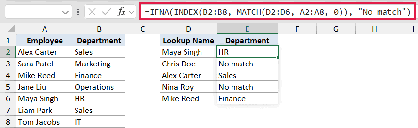
MATCH finds the position of each name from D2:D6 in the list A2:A8, and INDEX returns the department at that position. When a name like “Chris Doe” isn’t found, MATCH returns #N/A, which flows up through INDEX, and IFNA turns it into “No match”.
Just like Example 1, this spills down the whole column because I passed the range D2:D6 to MATCH.
Example 4: Return 0 So Totals Still Add Up
A blank message isn’t always what you want. Sometimes you need the missing values to become 0 so the rest of your math keeps working.
Below is a price list in columns A and B, and a list of ordered items in column D. Some of those items aren’t in the price list.
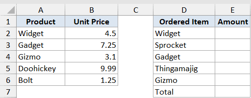
I want to pull each item’s amount into column E, and total them at the bottom. If an item isn’t found, it should count as 0 rather than breaking the total.
Here is the formula:
=IFNA(VLOOKUP(D2, $A$2:$B$6, 2, FALSE), 0)
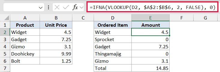
For items like “Sprocket” and “Thingamajig” that aren’t in the price list, VLOOKUP returns #N/A, and IFNA replaces it with 0. Without IFNA, even one #N/A in the column would make the SUM in cell E7 return #N/A too. With the zeros in place, the total adds up cleanly.
If you’re on Excel 365, you could also write the column in one spilling formula, =IFNA(VLOOKUP(D2:D6, $A$2:$B$6, 2, FALSE), 0), and total it with =SUM(E2#). The per-row version above works in every version of Excel.
Example 5: IFNA vs IFERROR
This is the most important thing to understand about IFNA. It catches only the #N/A error, not every error. That’s actually a feature, not a limitation.
Below is a column of formula results in column A. Some return #N/A (a failed lookup), and one returns #DIV/0! (a division by zero).
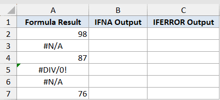
I want to compare what happens when I wrap these same results in IFNA versus IFERROR.
Here is the IFNA formula in column B:
=IFNA(A2, "Not Found")
And the IFERROR version in column C:
=IFERROR(A2, "Not Found")
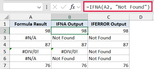
Look at the row with #DIV/0!. IFNA leaves it alone and still shows #DIV/0!, because that’s not an #N/A error. IFERROR, on the other hand, swallows it and shows “Not Found”, hiding the fact that something is actually wrong with that calculation.
That’s the key difference. Use IFNA when you specifically expect #N/A from a lookup and want every other error to stay visible. Use IFERROR only when you genuinely want to mask all errors.
Tips & Common Mistakes
- IFNA is not the same as IFERROR. IFNA catches only #N/A. IFERROR catches every error type (#DIV/0!, #VALUE!, #REF!, #NAME?, #NUM!, #NULL!, and #N/A). Reach for IFNA when a #N/A from a lookup is the only error you expect, so you don’t accidentally hide a genuine problem.
- IFNA needs Excel 2013 or later. It was added in Excel 2013. If you’re on an older version, you’ll need the longer ISNA pattern,
=IF(ISNA(...), value_if_na, ...), instead. - The fallback can be anything.
value_if_nadoesn’t have to be text. Use 0 for math, “” for a clean blank cell, or even another formula as a backup lookup. - In Excel 365, modern lookups often skip IFNA entirely. XLOOKUP has a built-in
if_not_foundargument, so=XLOOKUP(lookup, range, return, "Not Found")handles the missing case without IFNA. IFNA is still the right tool for VLOOKUP, HLOOKUP, and INDEX/MATCH formulas.
IFNA is one of those small functions that makes your spreadsheets a lot friendlier to read. It turns those jarring #N/A errors into something meaningful, whether that’s a message, a zero, or a blank. The big thing to remember is that it only touches #N/A, so the rest of your errors stay visible and you keep control over what gets hidden.
Related Excel Functions / Articles:
- LOOKUP Function in Excel
- VLOOKUP Not Working – 7 Possible Reasons + Fix!
- XLOOKUP Vs INDEX MATCH in Excel
- Bulk Find and Replace in Excel
- #REF! Error in Excel
- Using VLOOKUP Approximate Match in Excel (Examples)
- #VALUE! Error in Excel – How to Fix!
- Multiple If Statements in Excel (Nested IFs, AND/OR) with Examples
- IFERROR Function in Excel
