VLOOKUP Function in Excel (7 Easy Examples)

If you want to look up a value in one column of a table and pull back a matching value from another column, the VLOOKUP function is what you need.

It’s one of the most used functions in Excel, and once you get the four parts straight, it’s easy to work with.

In Excel 365, you can also give VLOOKUP a whole range of lookup values at once and the results spill into the cells below. In this article, I’ll walk you through how VLOOKUP works with seven practical examples, from a simple exact match to a multi-criteria lookup.

Table of Contents

VLOOKUP Function Syntax in Excel

The VLOOKUP function searches for a value in the first column of a range and returns a value from a column you specify in the same row.

=VLOOKUP(lookup_value, table_array, col_index_num, [range_lookup])

lookup_value – the value you want to find. VLOOKUP looks for this in the first column of your table.
table_array – the range that holds your data. The lookup column has to be the leftmost column of this range.
col_index_num – the column number to pull the result from, counting from the left of the table (the first column is 1).
range_lookup – optional. Use FALSE for an exact match, or TRUE for an approximate match. If you leave it out, Excel assumes TRUE.

When to Use VLOOKUP Function

VLOOKUP is handy any time you need to pull related information from a table based on a single key. Some common cases:

Find a price, salary, or status by an ID code.
Match a name to its email, phone number, or department.
Assign a grade, discount, or tax rate based on a number falling into a range.
Pull details from a master list into a smaller report or form.
Combine two sheets of data using a shared key like an order number.

Example 1: Exact Match Lookup

Let’s start with the most common use of VLOOKUP, an exact match.

Below is a small employee table with the ID, name, department, and salary for each person.

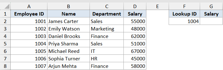
Vlookup Function Dataset Example 1 showing employee data table with columns for ID, Name, Department, and Salary

We want to find the salary for employee ID 1004.

Here is the formula:

=VLOOKUP(F2,A2:D8,4,FALSE)

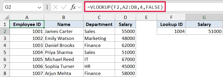
Excel formula bar showing a VLOOKUP function for an exact match, referencing an employee ID table to return a salary

The formula looks for the value in F2 (1004) in the first column of the range A2:D8. When it finds the matching row, it returns the value from the 4th column of that range, which is the Salary column.

The FALSE at the end tells VLOOKUP you want an exact match. So it returns 51000, the salary for Priya Sharma.

Pro Tip: The column number counts from the first column of your table_array, not from column A of the sheet. In this table the salary is the 4th column of A:D, so col_index_num is 4.

Example 2: Approximate Match for Tiers

Here’s a scenario where you actually want an approximate match instead of an exact one.

Below is a discount table. The left column lists the minimum order quantity for each tier, and the right column shows the discount that applies from that quantity up.

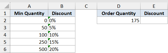
Vlookup Function Dataset Example 2 showing a discount table with minimum quantities and an order quantity of 175

We want to find the discount for an order of 175 units.

Here is the formula:

=VLOOKUP(D2,A2:B6,2,TRUE)

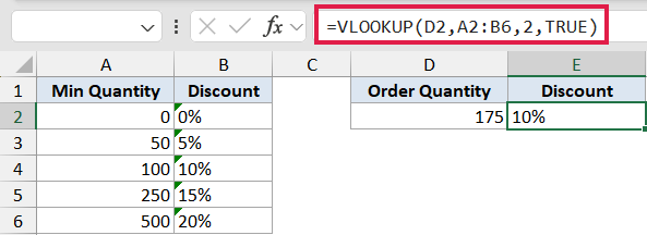
Excel formula bar displaying VLOOKUP with TRUE for approximate match, referencing a quantity-based discount table

With TRUE as the last argument, VLOOKUP doesn’t need an exact match. It finds the largest value that is still less than or equal to 175, which is 100, and returns the discount next to it.

So an order of 175 units lands in the 100 tier and gets a 10% discount.

Pro Tip: Approximate match only works correctly when the first column is sorted in ascending order. If your tiers are out of order, you’ll get wrong results without any error message.

Example 3: Look Up Many Values at Once

If you’re on Excel 365, you don’t have to copy VLOOKUP down one row at a time. You can hand it a whole range of lookup values in one go.

Below is a product list with IDs and prices on the left. On the right is a short list of product IDs we need prices for.

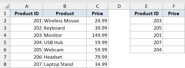
Vlookup Function Dataset Example 3 showing a product price reference table and a lookup table with empty price cells

We want to pull the price for every ID in the list E2:E6 with a single formula.

Here is the formula:

=VLOOKUP(E2:E6,A2:C8,3,FALSE)

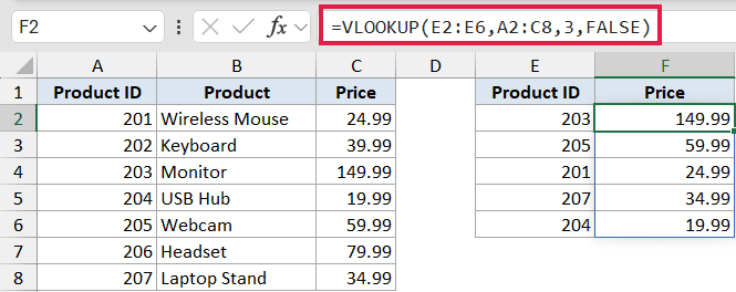
Excel formula bar showing VLOOKUP with an array reference for the lookup value, returning prices for product IDs

Instead of one lookup value, we passed the whole range E2:E6. VLOOKUP returns a price for each one and the results spill down into the cells below automatically.

You write the formula once in F2 and Excel fills the rest. There’s nothing to drag down.

Pro Tip: If the cells where the results need to spill aren’t empty, you’ll see a #SPILL! error. Clear the cells below the formula and the spill will appear.

Example 4: Handle Missing Values with IFERROR

When VLOOKUP can’t find a match, it returns an ugly #N/A error. You can replace that with a friendly message using IFERROR.

Below is a customer list on the left. On the right is a set of IDs we’re looking up, and some of them don’t exist in the list.

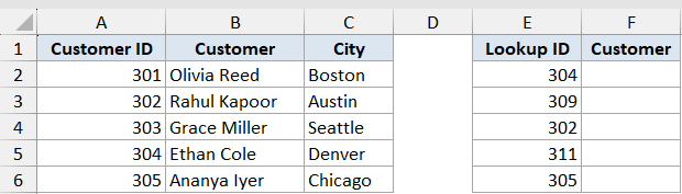
Excel dataset with Customer ID, Name, and City columns alongside a lookup table for Customer ID and empty Name column

We want the customer name for each ID, and a clean “Not found” message for any ID that isn’t in the list.

Here is the formula:

=IFERROR(VLOOKUP(E2:E6,$A$2:$C$6,2,FALSE),"Not found")

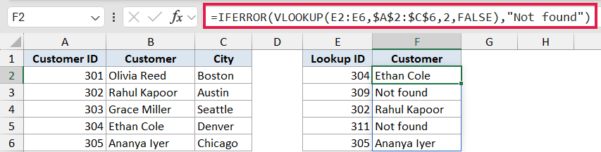
Excel formula bar showing IFERROR VLOOKUP function returning Not found for missing values in a customer lookup table

The VLOOKUP part still spills a result for each ID in E2:E6. IFERROR checks each one, and wherever VLOOKUP would have returned #N/A, it shows “Not found” instead.

So IDs 309 and 311 come back as “Not found” while the rest return their customer names.

In Excel 365 you can also do this with XLOOKUP, which has a built-in spot for the not-found message: =XLOOKUP(E2:E6,A2:A6,B2:B6,"Not found"). The IFERROR approach still works everywhere, so it’s worth knowing both.

Example 5: Partial Match with Wildcards

VLOOKUP can match on part of a text value when you wrap the lookup with wildcards.

Below is a contact list with full names and email addresses.

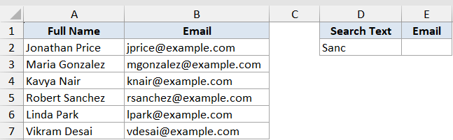
Vlookup Function Dataset Example 5 showing a name and email table with a search field for partial match lookup

We only remember part of a last name, “Sanc”, and we want to find that person’s email.

Here is the formula:

=VLOOKUP("*"&D2&"*",A2:B7,2,FALSE)

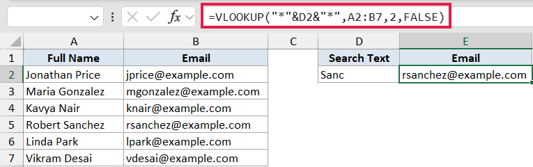
VLOOKUP formula using wildcards to find a partial match for email address in Excel table

The asterisk (*) is a wildcard that stands for any number of characters. By putting one before and after D2, we’re telling VLOOKUP to find any name that contains “Sanc” anywhere in it.

That matches “Robert Sanchez”, so the formula returns his email address.

Pro Tip: Use * to match any number of characters and ? to match a single character. Wildcards only work with an exact match, so keep the last argument set to FALSE.

Example 6: Lookup on Multiple Criteria

VLOOKUP only looks at one column, but you’ll often need to match on two things at once, like a region and a product together. The trick is a helper column.

Below is a sales table. Columns A and B hold the Region and Product, and column C is a helper column that joins them into a single key using =A2&B2. Column D has the units sold.

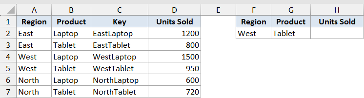
Excel dataset showing a source table with Region, Product, Key, and Units Sold columns alongside a lookup criteria table

We want the units sold for the West region’s Tablet, matching on both fields.

Here is the formula:

=VLOOKUP(F2&G2,C2:D7,2,FALSE)

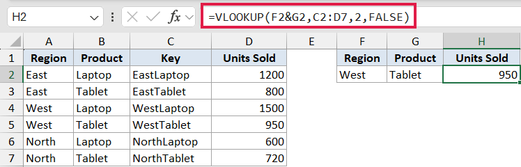
VLOOKUP formula using concatenated lookup value F2&G2 to find units sold in an Excel table

We join the two lookup values, F2 and G2, into “WestTablet” the same way the helper column was built. VLOOKUP then searches the helper column C for that combined key.

It finds the matching row and returns 950 from the units column. The helper column is what lets a single-column function match on two criteria.

Pro Tip: Make sure the helper column is the leftmost column of your table_array (here it’s column C, the start of C2:D7). VLOOKUP always searches the first column of the range you give it.

Example 7: Dynamic Column with MATCH

Typing the column number by hand gets tedious when your table is wide. You can let MATCH work out the column number for you.

Below is a quarterly sales table with one row per product and a column for each quarter.

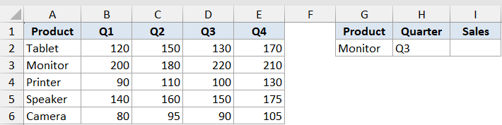
Excel dataset showing product sales by quarter with a lookup table for Monitor Q3 sales

We want the sales for a product and a quarter that we pick, here Monitor and Q3.

Here is the formula:

=VLOOKUP(G2,A2:E6,MATCH(H2,A1:E1,0),FALSE)

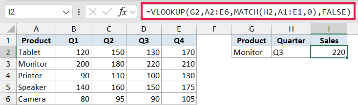
VLOOKUP formula using MATCH to dynamically find the column index for Monitor Q3 sales in an Excel table

How this formula works:

MATCH(H2,A1:E1,0) looks for “Q3” in the header row A1:E1 and returns its position, which is 4.
That 4 becomes the col_index_num for VLOOKUP.
VLOOKUP then finds “Monitor” in the first column and returns the value from the 4th column, 220.

Now you can change the product or the quarter and the formula adjusts on its own. No need to edit the column number every time.

Tips & Common Mistakes

VLOOKUP only looks to the right. The lookup column must be the leftmost column of your table_array, and the result has to be in a column to its right. If you need to look the other way, use INDEX/MATCH or XLOOKUP.
Lock your table range with absolute references. When you copy a VLOOKUP down, use $A$2:$D$8 so the table doesn’t shift. The lookup value usually stays relative.
The default match is approximate. If you forget the last argument, VLOOKUP uses TRUE and can return the wrong value on unsorted data. Get in the habit of always typing FALSE for exact matches.
A #N/A error usually means no match was found. Check for extra spaces, numbers stored as text, or a typo in the lookup value before assuming the formula is broken.
XLOOKUP is the modern alternative. If you’re on Excel 365, XLOOKUP can look left or right, doesn’t need a column number, and has a built-in not-found message. VLOOKUP is still worth knowing since it works in every version of Excel.

VLOOKUP is one of those functions that pays off the moment you learn it. Once you’re comfortable with exact and approximate matches, the rest is mostly combining it with other functions like IFERROR and MATCH.

Open one of your own tables and try a simple exact match first. The rest of these examples will make a lot more sense once you’ve done that one yourself.

List of All Excel Functions

Related Excel Functions / Articles: