If you want to generate random numbers in Excel, the RAND function is the quickest way to do it.
In this article, I’ll show you four practical examples of how to use RAND in your spreadsheets.
RAND returns one random value per cell and does not spill, so for a whole range of random numbers in one formula use its dynamic array cousin RANDARRAY.
RAND Function Syntax in Excel
Here is the RAND function syntax:
=RAND()
RAND takes no arguments. The parentheses stay empty. It returns a random decimal that is at least 0 and less than 1.
One thing to keep in mind: RAND is volatile. The value changes every time you edit a cell or press F9 to recalculate. More on that in the Tips section.
When to Use RAND Function
- Get a random decimal between 0 and 1.
- Scale the result to any custom range with the formula
=a + RAND()*(b-a), where a is the lower bound and b is the upper bound. - Add a helper column of random values to shuffle a list into a random order.
- Generate dummy or test data when you need placeholder numbers fast.
Example 1: Generate a Random Decimal
Let’s start with the most basic use of RAND.
Below is a list of six students. The goal is to assign each one a random decimal score between 0 and 1.
I want to fill column B with a random number for each student.
Here is the formula:
=RAND()
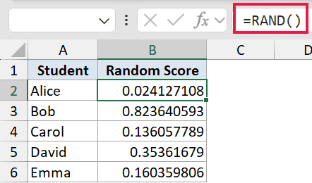
Enter =RAND() in cell B2 and copy it down to B6. Each cell calculates its own random decimal separately.
Note that any edit anywhere in the sheet will reshuffle every RAND value. That’s by design, but it can catch you off guard the first time it happens.
Pro Tip: To lock the numbers in place, select the cells, copy them (Ctrl+C), then use Paste Special > Values (Ctrl+Alt+V → V → Enter). You can also press F9 while you are still in the formula bar to freeze just that one cell before pressing Enter.
Example 2: Random Number Between Two Bounds
Here’s a more practical scenario: generating a random price within a specific range for each product.
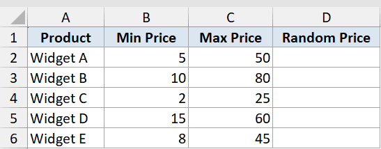
Below is a product list with a Min Price and Max Price for each item. I want a random price in column D that falls somewhere between those two bounds.
If you need numbers that don’t repeat, check out this guide on generating random numbers without duplicates in Excel.
I want to scale RAND into the custom range defined by each row’s Min and Max values.
Here is the formula:
=B2+RAND()*(C2-B2)
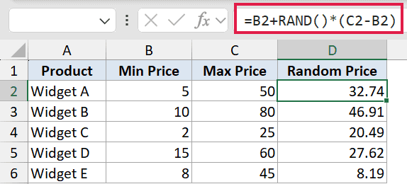
The formula takes RAND’s output (a number between 0 and 1) and stretches it across the gap between the Min and Max. Adding the Min then shifts the result into the right range.
Copy the formula down to D6 and each product gets its own random price within its own bounds.
Example 3: Random Integer (Priority 1 to 10)
Here’s a handy variation: getting a whole number instead of a decimal.
Here’s a task list with assignees in column B. I want a random priority score from 1 to 10 in column C for each row.
I want a whole number between 1 and 10, not a decimal.
Here is the formula:
=INT(RAND()*10)+1
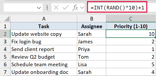
RAND()*10 gives a decimal between 0 and 10. INT chops off everything after the decimal point, leaving a whole number from 0 to 9. Adding 1 shifts the range to 1 to 10.
In modern Excel 365, =RANDBETWEEN(1,10) does the same thing in a cleaner way. And =RANDARRAY(6,1,1,10,TRUE) spills all six integers at once in a single formula, with no fill-down needed. The INT + RAND approach still works in older Excel versions where those functions aren’t available.
You can also use RAND with the CHOOSE function to randomly pick a value from a fixed list, like assigning team names to participants at random.
Example 4: Shuffle a List With a RAND Helper Column
This one comes in handy more often than you’d expect.
Below is a list of employees from different departments. I want to shuffle them into a random order, useful for raffle draws, randomized survey assignments, or training rosters.
I want to add a helper column of random keys so I can sort the list by those values to get a random order.
Here is the formula:
=RAND()
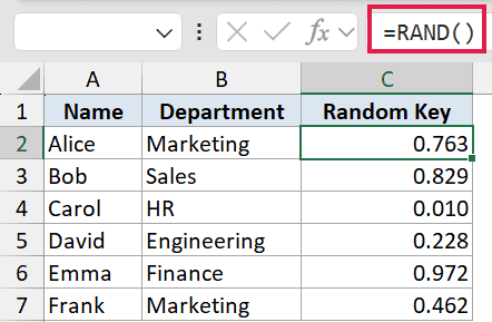
Enter =RAND() in C2 and copy it down to C7. Then sort the entire table by column C.
Each time you sort, the random keys shuffle the rows into a new order. After you get the order you want, paste the result as values so it stops reshuffling on every recalculation.
In Excel 365, you can skip the helper column entirely. =SORTBY(A2:B7,RANDARRAY(ROWS(A2:A7))) shuffles the whole list in one formula. Still paste as values afterward if you need the order to stay fixed.
RAND also works well for generating random test data like random dates or random letters when you combine it with the right wrapper formula.
Pro Tip: After sorting by the RAND helper column, immediately use Paste Special > Values on the sorted data to freeze the order. Otherwise the next keystroke recalculates RAND and quietly reshuffles your list.
Tips & Common Mistakes
- RAND recalculates on every edit. Press F9 or type anything in any cell and all your RAND values change. Copy and Paste Special > Values as soon as you want them to stay put.
- For random integers,
=RANDBETWEEN(1,10)is cleaner than=INT(RAND()*10)+1. It works in Excel 2010 and newer, so there’s usually no reason to use the longer form. - On Excel 365 or 2021,
=RANDARRAY(10,1)gives you ten random decimals in one formula. You can also pass it bounds and set the last argument to TRUE for whole numbers. - Each RAND call is completely separate from every other one. There’s no seed, no shared state. Two RAND formulas have no connection to each other.
- RAND never returns exactly 0 or 1. The result is always strictly between those two values, so
=RAND()*10will never land on exactly 0 or 10.
RAND is a small function that does one thing well. Once you get a feel for the volatility and remember to paste as values when the numbers need to stay put, it covers a lot of ground: test data, shuffling, random assignments, and more.
Related Excel Functions / Articles: