OR Function in Excel (6 Easy Examples)

If you want to check whether at least one of several conditions is true, the OR function in Excel is what you’re looking for. It returns TRUE if any condition you give it is met, and FALSE only when every condition fails.

OR returns a single value, but it works seamlessly inside dynamic array formulas like =SUM(FILTER(...)). In this article, I’ll show you how to use OR on its own, inside IF, and as part of a dynamic array.

Table of Contents

OR Function Syntax in Excel

The OR function checks one or more conditions and returns a single TRUE or FALSE.

=OR(logical1,[logical2],...)

logical1 – The first condition you want to test. This is required.
logical2, … – Additional conditions to test. These are optional. You can include up to 255 conditions in total.

Each condition is something that evaluates to TRUE or FALSE, like B2>=70 or C2="High".

When to Use OR Function

Here are some common situations where OR comes in handy:

Check if a row meets at least one of several rules (a high score OR enough bonus points).
Flag records that need attention when any single condition is hit.
Combine OR with IF to return readable text like “Pass” or “Resit” instead of TRUE/FALSE.
Mix text and number checks in the same test.
Build OR-style logic across a whole column inside FILTER or SUMPRODUCT.

Example 1: Test Multiple Conditions with OR

Let’s start with a simple example.

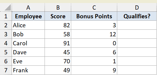
Below is the dataset with employee names, their scores, and bonus points earned.

Excel example 1 dataset showing employee names, scores, and bonus points with an empty Qualifies column for OR function

An employee qualifies if their score is 70 or higher, or if they earned 10 or more bonus points. We want a TRUE/FALSE flag in column D.

Here is the formula:

=OR(B2>=70,C2>=10)

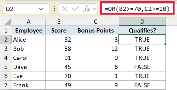
Excel formula =OR(B2>=70,C2>=10) in cell D2 showing Alice qualifies as TRUE

OR checks both conditions and returns TRUE if either one is met. Alice qualifies on her score of 82, and Bob qualifies on his 12 bonus points.

Dave fails both checks, so he gets FALSE. The formula is filled down from D2 to D7 so every employee gets a result.

Example 2: Wrap OR Inside IF for a Readable Result

Here’s a more practical scenario.

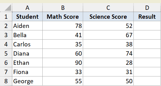
Below is the dataset showing students with their Math and Science scores.

Example 2 dataset showing student names, math scores, and science scores in an Excel table for OR function testing

A student passes if they score 50 or more in either subject. Instead of a bare TRUE/FALSE, we want the words “Pass” or “Resit” in column D.

Here is the formula:

=IF(OR(B2>=50,C2>=50),"Pass","Resit")

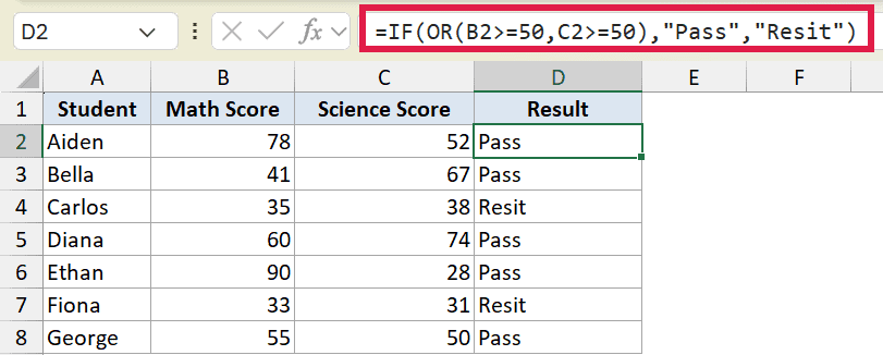
Excel formula bar showing IF OR function with result column displaying Pass or Resit based on student test scores

OR does the testing and IF turns the answer into readable text. If either score clears 50, OR returns TRUE and IF prints “Pass”.

Carlos scored 35 and 38, so both checks fail and he gets “Resit”. This IF + OR combo is the form you’ll reach for most often in real work.

Pro Tip: When you find yourself testing several “or” conditions, wrap OR inside IF so the result reads in plain language instead of TRUE/FALSE.

Example 3: Mix Text and Number Conditions

OR doesn’t care whether you’re checking text or numbers. You can mix both in the same formula.

Below is the dataset with order IDs, their region, and priority level.

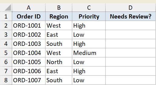
Example 3 dataset showing an Excel table with columns for Order ID, Region, Priority, and an empty Needs Review column

An order needs review if it’s from the West region or marked High priority. We want “Yes” or “No” in column D.

Here is the formula:

=IF(OR(B2="West",C2="High"),"Yes","No")

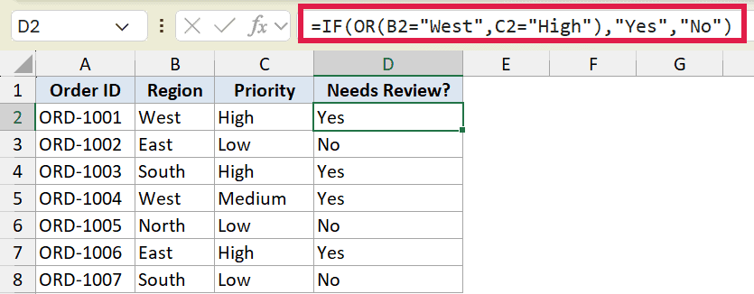
The first condition checks the region text, the second checks the priority text. If either matches, OR returns TRUE and IF prints “Yes”.

ORD-1002 is from the East with Low priority, so both checks fail and it gets “No”. Text comparisons in OR are not case sensitive, so “west” and “West” are treated the same.

Example 4: Combine OR with Comparison Operators

Let’s step it up with both a text match and a number comparison.

Below is the dataset showing support tickets, their status, and how many hours each has been open.

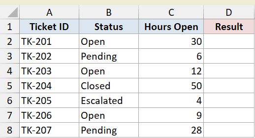
Excel dataset showing Ticket ID, Status, and Hours Open columns for OR function example 4

A ticket is urgent if its status is “Escalated” or it has been open more than 24 hours. We want TRUE or FALSE in column D.

Here is the formula:

=OR(B2="Escalated",C2>24)

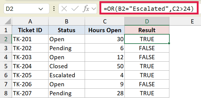
The >24 is a comparison operator that returns TRUE when the hours exceed 24. OR pairs that with the text check on the status.

TK-201 has been open 30 hours, so it returns TRUE even though its status is just “Open”. TK-205 is “Escalated” with only 4 hours open, and it still returns TRUE on the status match.

Example 5: Flag Items That Hit Any Rule

Here’s another flagging scenario, this time for inventory.

Below is the dataset with items, their category, and current stock count.

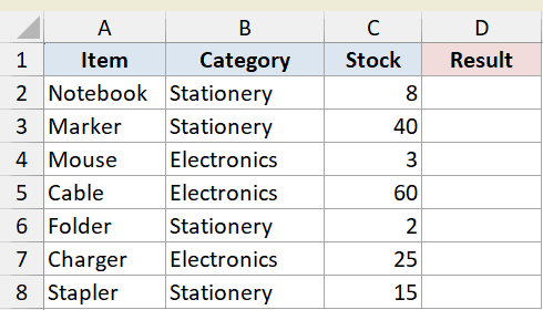
Example 5 dataset showing an Excel table with columns for Item, Category, and Stock, with an empty Result column

We want to flag an item if it’s in the Electronics category or its stock is below 5 units. The result goes in column D as TRUE or FALSE.

Here is the formula:

=OR(B2="Electronics",C2<5)

Excel formula bar showing OR function with criteria B2=

Every Electronics item gets flagged no matter the stock level, and any low-stock item gets flagged whatever its category. The Folder has only 2 in stock, so it returns TRUE even though it’s Stationery.

The Marker is Stationery with 40 in stock, so both conditions fail and it returns FALSE. This is the classic “flag anything that hits any rule” pattern.

Example 6: Use OR Logic Inside a Dynamic Array

Now let’s use OR-style logic across a whole range inside a dynamic array.

Below is the dataset with sales reps, their region, and sales figures.

Example 6 dataset in Excel showing sales representatives, regions, and sales figures in columns A through C

We want the total sales for reps in the West or East region, all in a single cell. The OR function itself collapses a whole column to one TRUE/FALSE, so it can’t filter row by row here.

Here is the formula:

=SUM(FILTER(C2:C7,(B2:B7="West")+(B2:B7="East")))

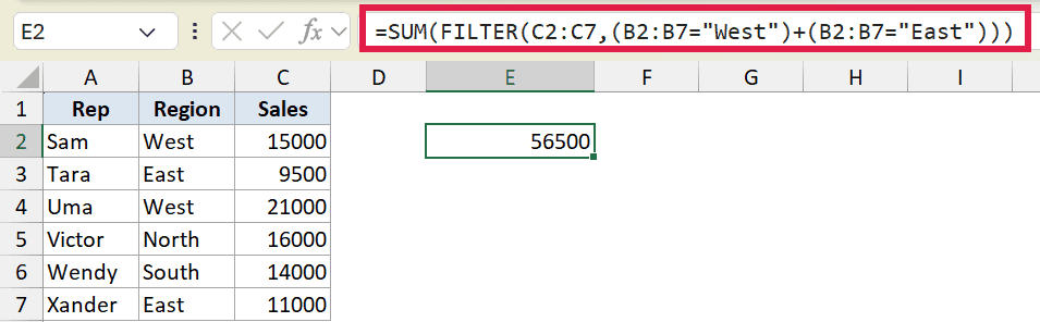
Excel formula using SUM and FILTER to calculate a total for West or East regions, resulting in 56500

The trick is the addition sign between the two conditions. Adding two TRUE/FALSE arrays gives you 1 where either condition is met, which is OR logic applied across every row.

FILTER keeps only the West and East rows, then SUM adds their sales. This additive pattern is how you get OR behaviour inside FILTER, SUMPRODUCT, and similar functions.

Pro Tip: Inside dynamic array formulas, use `+` between conditions for OR logic and `*` for AND logic. The plain OR function only returns one value, so it can’t filter a range on its own.

Tips & Common Mistakes

OR returns TRUE when at least one condition is met. It only returns FALSE when every single condition fails. If you need TRUE only when exactly one condition is met, use the XOR function instead.
You can test up to 255 conditions in one OR function, so there’s plenty of room for complex checks.
If a referenced range contains no logical values at all (only text or blanks), OR can return a #VALUE! error. Make sure your conditions actually evaluate to TRUE or FALSE.
Text comparisons in OR are not case sensitive. “Yes”, “YES”, and “yes” all match the same way.
To apply OR logic across a whole range (not just one row), don’t use the OR function. Use additive criteria like (range="a")+(range="b") inside FILTER or SUMPRODUCT instead.

That covers the OR function, from a simple multi-condition check to wrapping it inside IF and applying OR logic across a whole range in a dynamic array. In day-to-day work the IF + OR combination is the one you’ll reach for most.

So pick the form that fits your data. Use OR on its own when you just need TRUE/FALSE, and wrap it in IF when you want readable text instead.

List of All Excel Functions

Related Excel Functions / Articles: