
If you want to know what share of your data falls into each group, relative frequency is the number you’re after. It turns raw counts into proportions, so a busy day and a slow day become easy to compare at a glance.
Excel doesn’t have a single “relative frequency” button, which trips up a lot of people. The good news is you only need a short formula or a couple of clicks in a PivotTable.
In this tutorial I’ll show you three ways to build a relative frequency table, from a simple formula to a no-formula PivotTable.
Method #1: Using a COUNTIFS Formula
COUNTIFS counts how many values fall between a lower and an upper limit. Divide that count by the total number of days, and you get the relative frequency for that bin.
This is the most transparent method of the three, because you can see exactly what is being counted. It’s the one I reach for first.
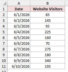
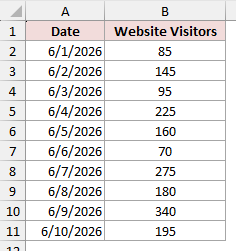
Below I have website visitor counts for 10 days. I want to group them into traffic bins of 100 and find what fraction of days lands in each bin.
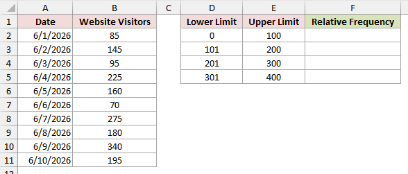
Next to the data I set up a small bin table with a Lower Limit column, an Upper Limit column, and an empty Relative Frequency column.
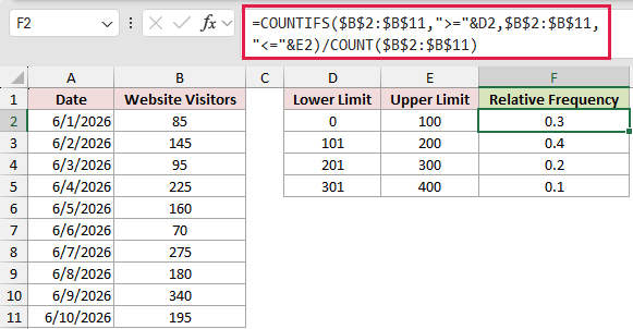
Here is the formula I put in the first Relative Frequency cell:
=COUNTIFS($B$2:$B$11,">="&D2,$B$2:$B$11,"<="&E2)/COUNT($B$2:$B$11)
Copy it down all four bins and each one fills in. The results come out as 0.3, 0.4, 0.2, and 0.1.
How does this formula work?
The COUNTIFS part counts the days where visitors are greater than or equal to the lower limit (D2) and less than or equal to the upper limit (E2). For the first bin that’s every day between 0 and 100, which is 3 days.
COUNT($B$2:$B$11) returns the total number of days, which is 10. Dividing 3 by 10 gives 0.3, the relative frequency for that bin.
The dollar signs lock the data range and the total, so the formula keeps pointing at the right cells as you copy it down the bin table.
Apply Percentage formatting and the same table reads as 30%, 40%, 20%, and 10%.
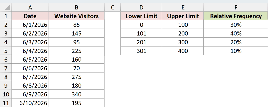
Note: The results show as decimals like 0.3 at first. Select the Relative Frequency cells and press Ctrl+Shift+% to apply Percentage formatting, and 0.3 becomes 30%. Microsoft documents this shortcut for the US keyboard layout, so use Percent Style on the Home tab if your keyboard differs.
Method #2: Using the FREQUENCY Function
Here’s a faster route if you’d rather fill the whole table with one formula instead of one bin at a time.
The FREQUENCY function counts how many values fall at or below each cutoff you give it, and it returns the whole set of counts in one go. Divide that by the total count and you get every relative frequency at once.
I’ll use the same 10 days of visitor data.
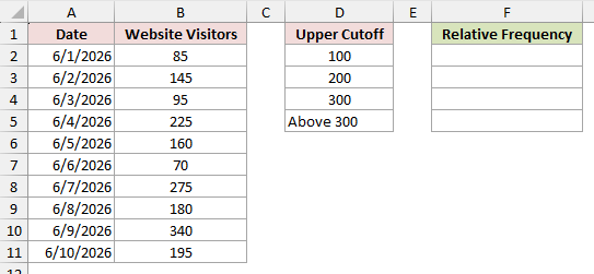
In a separate column I list the upper cutoffs for my bins: 100, 200, and 300.
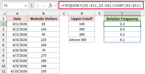
Here is the formula:
=FREQUENCY(B2:B11,D2:D4)/COUNT(B2:B11)
How does this formula work?
FREQUENCY takes the visitor data (B2:B11) and the three cutoffs (D2:D4). It returns four values: the count at or below 100, the count between 101 and 200, the count between 201 and 300, and everything above 300.
In Microsoft 365 the formula spills down automatically into those four cells, so one entry fills the whole table. Dividing each count by COUNT(B2:B11) turns the four counts (3, 4, 2, 1) into 0.3, 0.4, 0.2, and 0.1.
FREQUENCY always returns one more value than the number of cutoffs. That extra fourth value is the overflow bin, catching any day above your top cutoff of 300.
Format the spilled cells as percentages and you get 30%, 40%, 20%, and 10%, the same table as before.
Note: In Excel 2019 or earlier the formula won’t spill. Select four empty cells first, type the formula, and press Ctrl+Shift+Enter to enter it as an array. If you see a #SPILL! error in Microsoft 365, clear the cells directly below the formula so it has room to fill.
Method #3: Using a PivotTable
If you’d rather not write any formulas at all, a PivotTable can bin the data and show each bin’s share of the total for you.
The trick is to group the visitor counts into equal-width bins, then switch the values to show as a percentage of the grand total. There’s no formula to maintain.
I’m working with the same 10 days of visitor data.
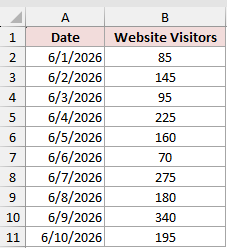
Here are the steps to build a relative frequency table with a PivotTable:
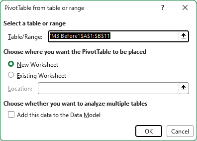
- Select any cell in the data, then on the Insert tab click PivotTable and choose New Worksheet.
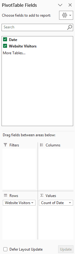
- In the PivotTable Fields pane, drag Website Visitors into the Rows area, then drag Date into the Values area. Date shows as Count of Date, which is the number of days.
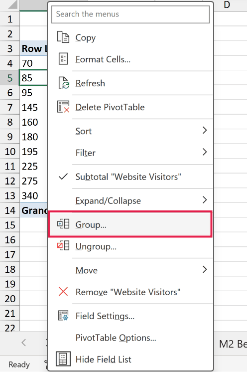
- Right-click any visitor number in the Rows column and choose Group.
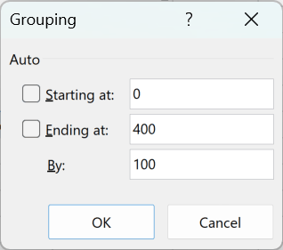
- In the dialog, type 0 in Starting at, 400 in Ending at, and 100 in By, then click OK.
The visitor counts are now grouped into bins of 100, and each bin shows the number of days in it.
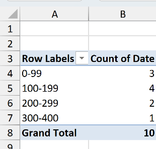
- Right-click any number in the Count of Date column, choose Value Field Settings, open the Show Values As tab, pick % of Grand Total, and click OK.
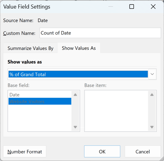
Each bin now shows its share of the grand total. The 100-199 bin holds 40% of the days, which matches what the formulas gave us.
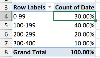
The PivotTable labels the bins as 0-99, 100-199, and so on, so they read a little differently from the 0-100 and 101-200 labels in the earlier methods.
Since no day sits exactly on a boundary like 100 or 200, every bin holds the same days and the percentages come out identical.
Note: When you open the Group dialog, Excel pre-fills Starting at and Ending at with the smallest and largest values in your data. Overwrite them with 0 and 400 so your bins start at a clean number. The percentages also show with two decimals by default (30.00%); use Decrease Decimal on the Home tab if you’d rather see 30%.
Additional Notes About Relative Frequency in Excel
- Your relative frequencies should always add up to 1 (or 100%). If they don’t, check that your bins cover every value with no gaps and no overlap.
- Keep the bins the same width. All four here span 100 visitors, which keeps the comparison between bins fair.
- COUNTIFS and FREQUENCY recalculate the moment your data changes, but a PivotTable does not. After editing the source data, right-click the PivotTable and choose Refresh.
- If Excel says “Cannot group that selection” when you try to group the pivot, the visitor column has a blank or a text entry in it. Clean those up and try again.
- If you just want the answer without building a table, this relative frequency calculator works it out from a plain list of counts.
Frequently Asked Questions
What’s the difference between frequency and relative frequency?
Frequency is the raw count of values in each bin, like 4 days in the 101-200 group. Relative frequency divides that count by the total, so the same bin becomes 0.4, or 40% of all days.
How do I calculate cumulative relative frequency in Excel?
Add a running total next to your relative frequency column. If the relative frequencies sit in F2:F5, put =SUM($F$2:F2) in the next column and copy it down. The values build to 30%, 70%, 90%, and finally 100%.
Can I turn a relative frequency table into percentages automatically?
Yes. Select the relative frequency cells and press Ctrl+Shift+%, or pick Percentage from the number format list on the Home tab. Only the display changes; the underlying decimal stays the same.
Conclusion
Relative frequency is just each bin’s count divided by the total, and Excel gives you three clean ways to get there.
Reach for the COUNTIFS formula when you want to see exactly what’s being counted, use FREQUENCY when you want the whole table from one formula, and use a PivotTable when you’d rather not write any formula at all.
Other Excel articles you may also like:
