
Excel’s COLUMN function returns the column number of a cell reference. Without a reference, it returns the column number of the cell containing the formula.
It is useful for formulas that change as you copy them across a worksheet. To count how many columns a range contains, use COLUMNS instead.
In this article, I’ll show you how to generate column numbers, build a flexible VLOOKUP, and sum every other column.
COLUMN Function Syntax in Excel
COLUMN takes an optional cell or range reference. This example uses cell F1 as that reference:
=COLUMN(F1)
referenceis optional. It is the cell or range whose column number you want.- If you omit
reference, COLUMN returns the column number of the cell containing the formula. - When
referenceis a range, Excel 365 can return several column numbers as a horizontal spill.
When to Use the COLUMN Function
- Find the numeric position of a particular worksheet column.
- Create counters that follow columns across a worksheet.
- Supply changing column index numbers to lookup formulas.
- Identify alternating columns for calculations or conditional formatting.
- Convert a column letter into its corresponding number.
Example 1: Get a Cell’s Column Number
Let’s start with the two basic ways to use COLUMN.
Below is the dataset with seven fields for IT service tickets, including hours, rates, and ticket status.
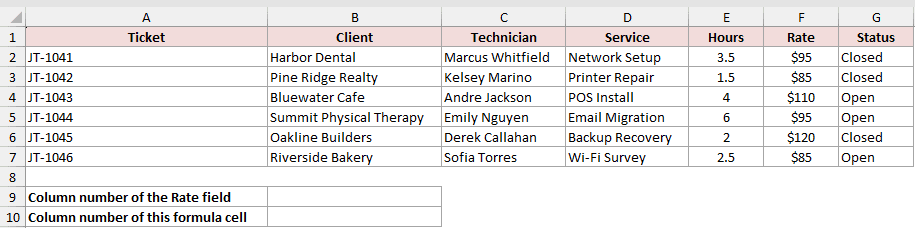
I want to find the column number of the Rate field in cell F1.
Here is the formula:
=COLUMN(F1)
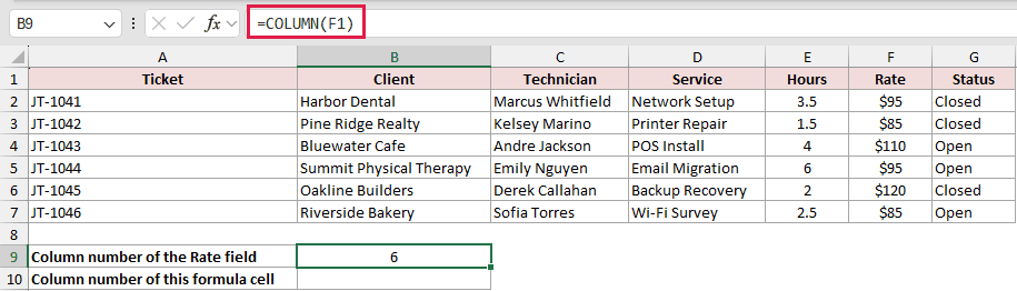
The formula returns 6 because column F is the sixth column on the worksheet.
You can also omit the reference and let COLUMN report the position of its own cell.
Here is the formula:
=COLUMN()
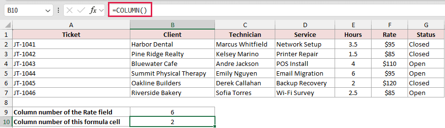
This formula sits in B10, so it returns 2. Moving it to another column would change the result.
Pro Tip: COLUMN reports worksheet positions, not positions within your dataset. A field in column F returns 6 even if your table starts in column D.
Example 2: Number Columns With a Spill Formula
Here’s a quick way to number several columns at once.
Below is the dataset with six work crews and their recorded hours from Monday through Saturday.
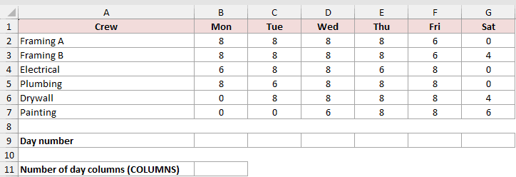
I want to place the numbers 1 through 6 below the six day columns.
Here is the formula:
=COLUMN(B1:G1)-1
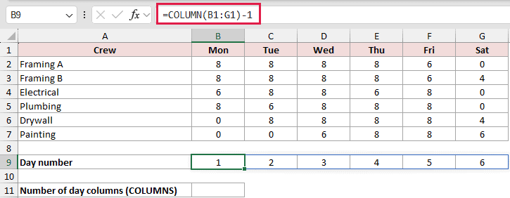
COLUMN first returns the worksheet positions 2 through 7 for columns B through G. Subtracting 1 changes those results to 1 through 6.
The single formula in B9 spills across B9:G9, so you do not need to copy it across the row.
If you only need the number of columns, use the COLUMNS function instead.
Here is the formula:
=COLUMNS(B1:G1)
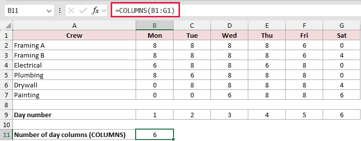
COLUMNS returns one result, 6. COLUMN returns the individual positions, which is why the first formula creates six values.
In Excel 365, =SEQUENCE(1,6) creates the same 1-through-6 counter with a shorter formula. The COLUMN version still works and can stay tied to a specific header range.
Pro Tip: Keep B9:G9 empty before entering the spilling formula. Any existing value in that area causes a #SPILL! error.
Example 3: Use COLUMN With VLOOKUP
COLUMN can also make a lookup return several fields.
Below is the dataset with vendor codes, vendor names, contacts, phone numbers, and payment terms. Cell G2 contains the code to find.

I want to return all four details for vendor code V-204 with one formula.
Here is the formula:
=VLOOKUP(G2,A2:E7,COLUMN(B1:E1),FALSE)

COLUMN(B1:E1) produces the column index numbers 2, 3, 4, and 5. VLOOKUP uses those numbers to return four fields from the matching row.
The results spill across H2:K2: Cascade Label Works, Renee Fitzgerald, (503) 555-0163, and Net 30.
In Excel 365, =XLOOKUP(G2,A2:A7,B2:E7) does this more directly because it needs no column index numbers. The VLOOKUP form still works in older versions.
Example 4: Sum Every Other Column
Let’s use each column’s relative position to pick alternating values.
Below is the dataset with quarterly sales and returns in alternating columns for six stores, followed by a Total Returns column.

I want to total only the four Returns columns for each store.
Here is the formula:
=SUMPRODUCT((MOD(COLUMN(B2:I2)-COLUMN($B$2)+1,2)=0)*B2:I2)
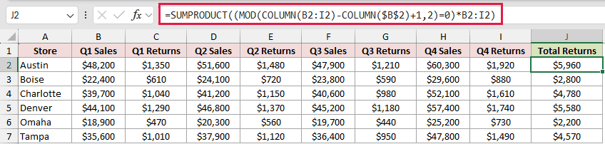
COLUMN(B2:I2)-COLUMN($B$2)+1 creates relative positions 1 through 8. MOD returns 0 for even positions, and the =0 test turns those results into TRUE.
Those even positions correspond to the four Returns columns. SUMPRODUCT multiplies the row values by that test and adds the selected amounts.
For Austin, the result is $5,960. Copying the formula down produces $2,800 for Boise and $4,780 for Charlotte.
In Excel 365, =SUM(CHOOSECOLS(B2:I2,2,4,6,8)) is easier to read. The SUMPRODUCT version still works where CHOOSECOLS is unavailable.
Example 5: Convert Column Letters to Numbers
Finally, let’s convert column letters stored as text.
Below is the dataset with report field names and their assigned column letters, including K, AB, AF, BZ, M, CD, and T.
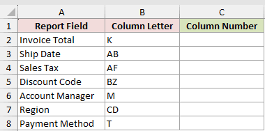
I want to return the numeric position for each stored column letter.
Here is the formula:
=COLUMN(INDIRECT(B2&"1"))
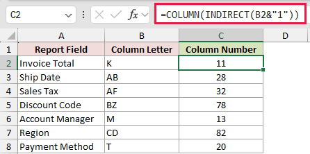
B2&"1" joins the letter K with row number 1, producing the text K1. INDIRECT turns that text into a cell reference.
COLUMN returns 11 for K. Fill the formula down to get the number for each remaining letter.
Pro Tip: INDIRECT is volatile, so Excel recalculates it whenever the workbook recalculates. Avoid using thousands of these formulas in a large workbook.
Tips & Common Mistakes
- COLUMN cannot use a reference made from multiple separate areas. Give it one cell or one continuous range.
- In Excel 365, adding
@before COLUMN forces implicit intersection and reduces a range result to one value. - A spilling COLUMN formula needs empty cells across its output area. Clear anything blocking that range if you see #SPILL!.
- In older Excel versions, a normal range formula returns only the leftmost column number. For all results, select the output range and press Ctrl + Shift + Enter.
- For alternating column shading, use
=MOD(COLUMN(),2)=0as a conditional formatting formula.
COLUMN works best when you know whether you need one column position or a spilled set of positions.
I hope you found this article helpful.
Related Excel Functions / Articles:
Other Excel articles you may also like:
