
Excel’s ROWS function returns the number of rows in a reference or array.
It measures the size of the range, including blank rows. That makes it useful for counting the height of a result or building formulas that expand with a range.
In this article, I’ll show you how to count filtered results and unique values, create serial numbers, and reverse a list.
ROWS Function Syntax in Excel
The ROWS function takes one range or array and returns its number of rows.
=ROWS(array)
- array (required) is the range or array whose rows you want to count. It can be a cell range, an array formula, or an array constant.
When to Use ROWS Function
- Count how many rows a fixed range contains, even when some cells are blank.
- Create serial numbers that adjust when you insert or delete worksheet rows.
- Count the records returned by FILTER or the distinct entries returned by UNIQUE.
- Supply a changing position number to INDEX as a formula moves down a column.
- Calculate the total cells in a rectangular range by multiplying ROWS by COLUMNS.
Example 1: Count Rows in a Range
Let’s start with a direct row count and compare it with two related calculations.
Below is the dataset. Columns A through D contain 12 shipment records, including the carrier, destination, and weight.
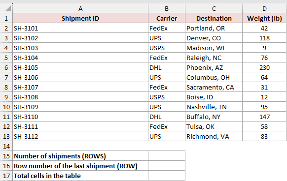
We want to count the shipment rows, identify the last worksheet row, and calculate the number of cells in the table.
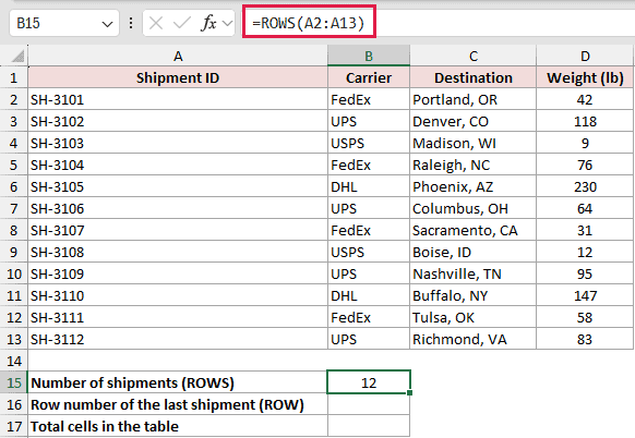
Here is the formula that counts the shipment rows:
=ROWS(A2:A13)
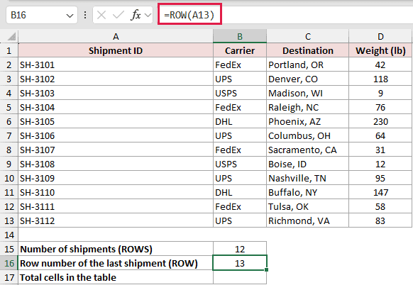
For comparison, this ROW formula returns the worksheet row number of the final shipment:
=ROW(A13)
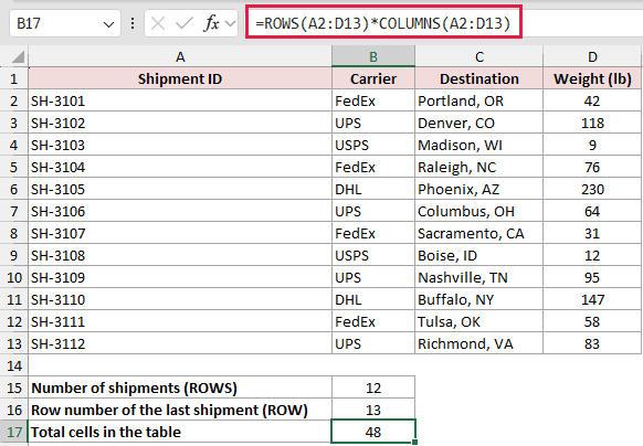
To count every cell in the four-column table, multiply the row count by the column count:
=ROWS(A2:D13)*COLUMNS(A2:D13)
The first formula returns 12 because A2:A13 contains 12 rows. ROW returns 13 because A13 sits on worksheet row 13.
The final formula multiplies 12 rows by four columns and returns 48 cells.
Pro Tip: ROWS counts the rows in a reference, not the nonblank cells. For example, =ROWS(A2:A13) still returns 12 if one shipment cell is empty.
Example 2: Generate Deletion-Safe Serial Numbers
Here’s a numbering method that updates when the list changes.
Below is the dataset. Column B lists 10 volunteers, column C shows their shifts, and column A is ready for serial numbers.
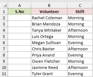
We want to number the volunteers from 1 to 10 without typing the sequence manually.
Enter this formula in A2 and copy it down through A11:
=ROWS($A$2:A2)
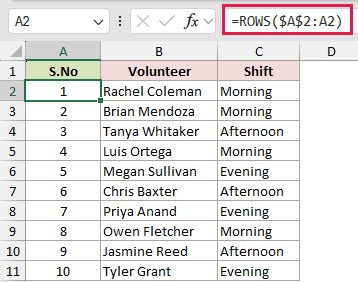
In A2, the expanding reference contains one row, so the formula returns 1. As the formula moves down, its lower endpoint changes while $A$2 stays fixed.
By A11, the reference contains 10 rows and returns 10. If you delete a volunteer row, the formulas below move up and the numbering closes automatically.
In Excel 365, =SEQUENCE(ROWS(B2:B11)) can spill the complete sequence from one formula. ROWS still determines how many serial numbers SEQUENCE should create.
Example 3: Count Rows Returned by FILTER
When a FILTER result can change size, ROWS can count the matching records.
Below is the dataset. Columns A through D contain 12 work orders, while F2 and G2 hold the Plumbing and Open criteria.
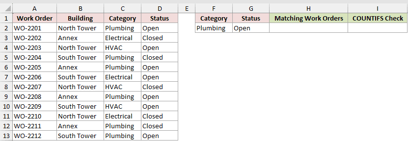
We want to count work orders where the category is Plumbing and the status is Open.
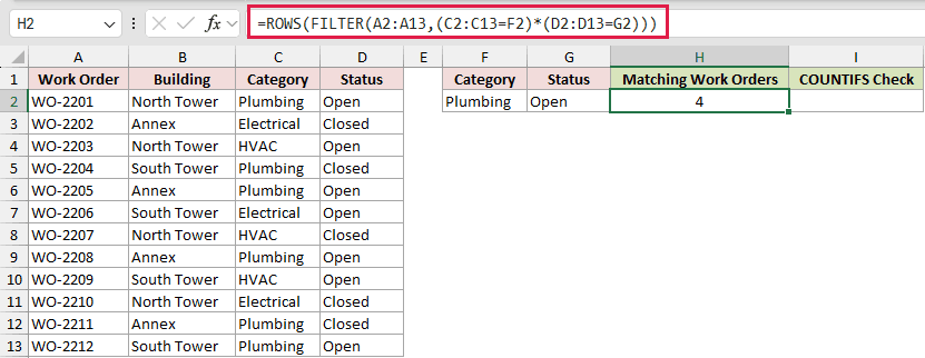
Here is the ROWS and FILTER formula in H2:
=ROWS(FILTER(A2:A13,(C2:C13=F2)*(D2:D13=G2)))
And here is the COUNTIFS formula in I2 for comparison:
=COUNTIFS(C2:C13,F2,D2:D13,G2)
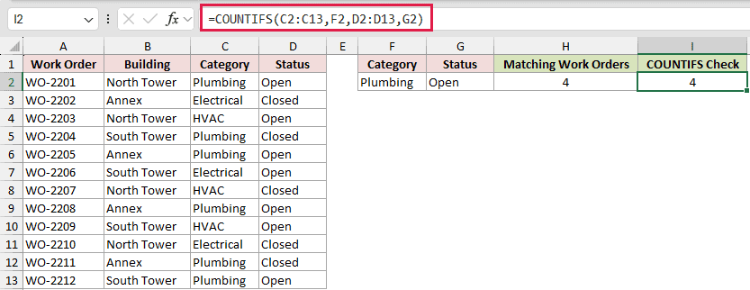
FILTER returns the matching work order IDs from column A. ROWS then counts those returned records and returns 4.
The matches are WO-2201, WO-2205, WO-2208, and WO-2212. COUNTIFS also returns 4 and is simpler for plain equality criteria.
ROWS with FILTER becomes more useful when your conditions are expressions that COUNTIFS cannot handle directly.
Pro Tip: FILTER returns #CALC! when nothing matches. Use =IFERROR(ROWS(FILTER(A2:A13,(C2:C13=F2)*(D2:D13=G2))),0) when you want a zero instead.
Example 4: Count Unique Values with ROWS
A list with repeated names is a good fit for UNIQUE and ROWS.
Below is the dataset. Columns A through C contain 12 gym classes, including repeated instructor names, while columns E and F hold the results.
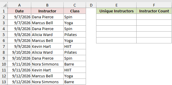
We want to create a unique instructor list and count how many instructors it contains.
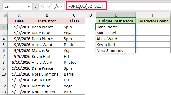
First, enter this formula in E2 to return the distinct names:
=UNIQUE(B2:B13)
Then use this formula in F2 to count that unique array:
=ROWS(UNIQUE(B2:B13))
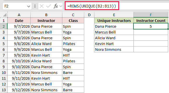
UNIQUE spills Dana Pierce, Marcus Bell, Alicia Ward, Kevin Hart, and Nora Simmons into E2:E6. Wrapping the same array in ROWS returns 5 in F2.
You could also use =COUNTA(UNIQUE(B2:B13)). ROWS states the intent more directly because you’re counting the rows in the returned array.
Example 5: Reverse a List with INDEX and ROWS
Finally, let’s use a shrinking row count to read a list from bottom to top.
Below is the dataset. Column A contains eight outbound bus stops, while column B will show the stops in reverse for the return trip.
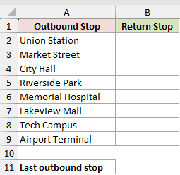
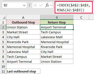
We want to reverse the route in B2:B9 and return the final outbound stop separately in B11.
Enter this formula in B2 and copy it down through B9:
=INDEX($A$2:$A$9,ROWS(A2:$A$9))
To return only the final outbound stop, use this formula in B11:
=INDEX(A2:A9,ROWS(A2:A9))
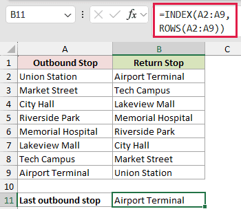
In B2, ROWS(A2:$A$9) returns 8, so INDEX returns the eighth stop, Airport Terminal. The row count falls by one as the formula moves down.
The copied formulas finish with Union Station in B9. The B11 formula counts all eight rows and returns Airport Terminal as the last value.
In Excel 365, =SORTBY(A2:A9,SEQUENCE(8),-1) can reverse the full list with one spilling formula. To return only the last value, use =TAKE(A2:A9,-1).
Tips & Common Mistakes
- ROWS counts every row in its reference, including blank rows. Use COUNTA when you need to count nonblank cells instead.
- ROWS includes rows hidden by AutoFilter. To count only visible AutoFiltered rows, use SUBTOTAL or AGGREGATE instead.
- ROWS and ROW answer different questions. ROWS returns the size of a reference, while ROW returns a cell’s worksheet row number.
- Lock the starting cell in expanding references such as
=ROWS($A$2:A2). Without the absolute reference, every copied formula would count only one row. - A ROWS formula returns one number and does not spill. It can still count a spilled array with a formula such as
=ROWS(E2#). - FILTER needs special handling when no records match. Wrapping ROWS and FILTER in IFERROR lets you return zero instead of #CALC!.
ROWS is handy whenever another formula needs to know the size or changing position of a range.
Revisit Example 2 for deletion-safe numbering, or Example 3 when you need to count filtered results.
Related Excel Functions / Articles:
- COUNT Function in Excel
- How to Count Unique Values in Excel (Formulas)
- Row vs Column in Excel – What’s the Difference?
Other Excel articles you may also like:
