
If you want to total one column using conditions stored in worksheet cells, the DSUM function is built for that job.
In this article, I’ll show you how to use DSUM with single criteria, multiple conditions, comparison operators, wildcards, and OR logic.
DSUM returns a single number, but it cannot use a FILTER result because its database and criteria must be worksheet ranges.
DSUM Function Syntax in Excel
The DSUM function adds values from one column when records match conditions in a separate criteria range.
=DSUM(database, field, criteria)
- database is the full list, including the header row. Each column is a field, and each row below the headers is a record.
- field identifies the column to total. You can use its quoted header, its position within the database, or a cell containing the header.
- criteria is a worksheet range containing at least one matching column header and one cell below it for the condition.
When to Use DSUM Function
- Build reports where someone can change conditions in worksheet cells without editing the formula.
- Apply several conditions with AND logic by placing them on the same criteria row.
- Add records matching any of several alternatives by placing those alternatives on separate criteria rows.
- Reuse one criteria range with DSUM and other database functions.
Example 1: Sum Labor for One Vehicle Type
The work-order sheet is a good place to see the basic three-part setup.
Below is the dataset. Columns A through D contain ten work orders, while the right-hand panel holds the Vehicle Type criterion.
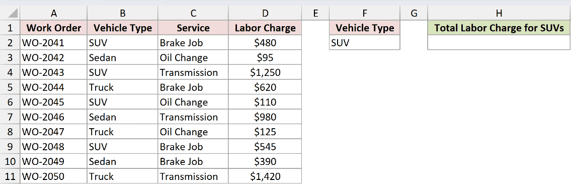
We want to total the labor charges for records where Vehicle Type is SUV.
Here is the formula:
=DSUM(A1:D11,"Labor Charge",F1:F2)
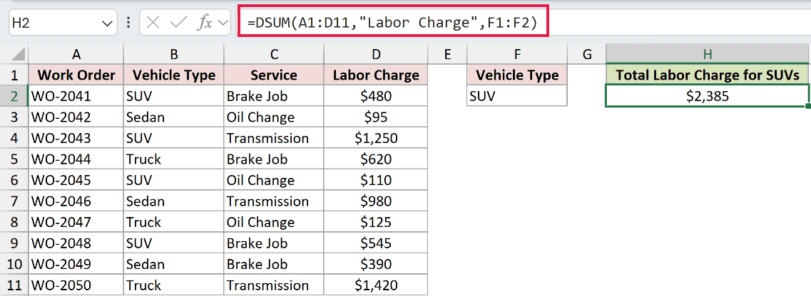
The database range includes the headers in row 1. The field argument names Labor Charge, and F1:F2 supplies the matching header and criterion.
Excel adds the four SUV charges and returns $2,385.
For this one-condition total, SUMIF is shorter. DSUM becomes more useful when the visible criteria range is reused or edited.
Pro Tip: Text criteria use begins-with matching. To force an exact match, enter a criterion that displays as =SUV.
Example 2: Use DSUM With AND Criteria
This veterinary invoice sheet shows how one criteria row narrows the total.
Below is the dataset. Columns A through D contain ten visits, with the veterinarian and visit type criteria placed to the right.
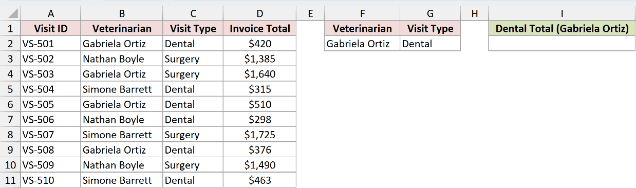
We want the total for dental visits handled by Gabriela Ortiz.
Here is the formula:
=DSUM(A1:D11,"Invoice Total",F1:G2)
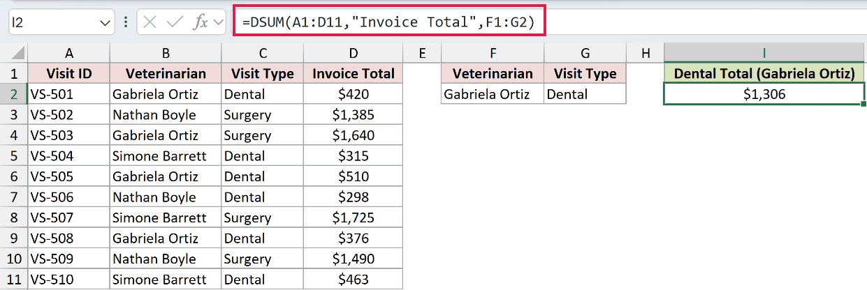
The two conditions share row 2, so DSUM treats them as AND criteria. A record must match both Gabriela Ortiz and Dental.
The three matching invoices total $1,306.
For straightforward AND conditions, SUMIFS is shorter. DSUM is useful when you want the conditions visible and editable on the worksheet.
Example 3: Use a Comparison Operator and Field Number
Purchase orders make the numeric test easy to see before the field argument changes to a number.
Below is the dataset. Columns A through D list ten purchase orders, while the right-hand criteria panel contains the Line Total condition greater than 1000.
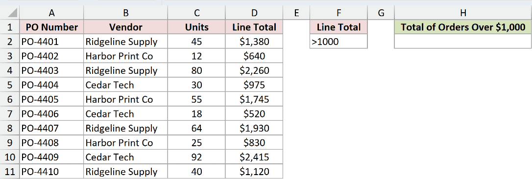
We want to add Line Total values above $1,000 using the field’s column position.
Here is the formula:
=DSUM(A1:D11,4,F1:F2)
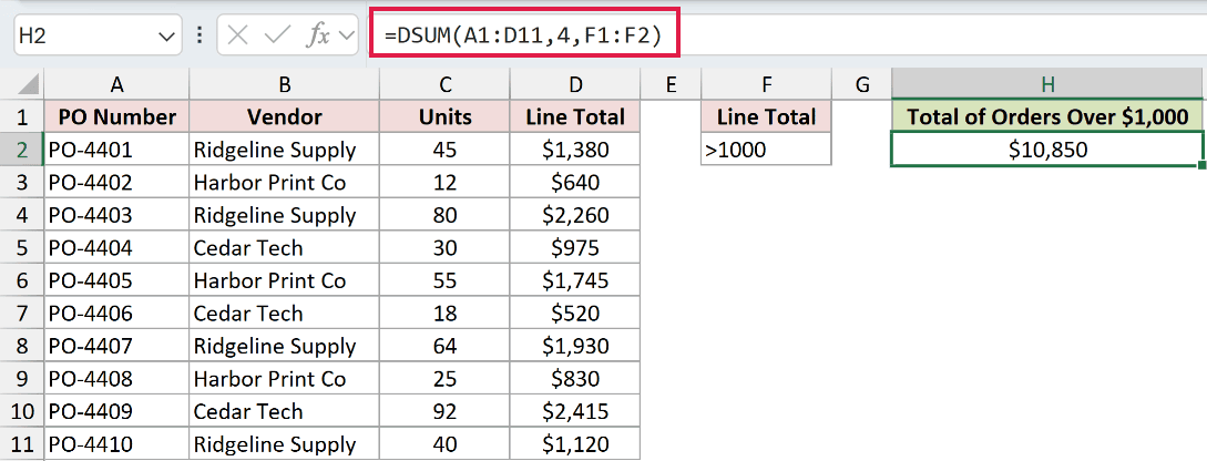
The field argument is 4, so DSUM totals the fourth column within A1:D11. The text in F2 applies the greater-than condition.
Six purchase orders qualify, producing a total of $10,850.
You can type operators such as greater than, less than, or not equal directly into a criteria cell with the comparison value.
Example 4: Use DSUM With OR Criteria
A donation log shows why separate criteria rows are handy.
Below is the dataset. Columns A through D contain ten donations, and the right-hand criteria panel lists two campaign names on separate rows.
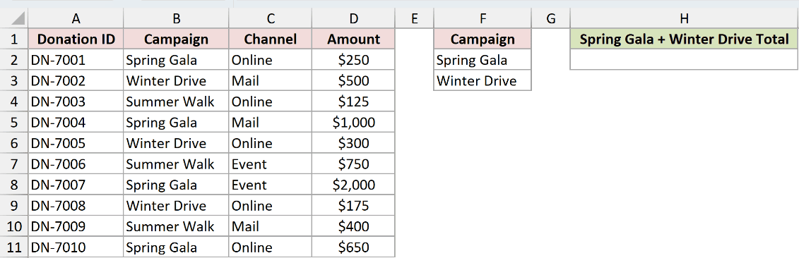
We want one total for the Spring Gala or Winter Drive campaigns.
Here is the formula:
=DSUM(A1:D11,D1,F1:F3)
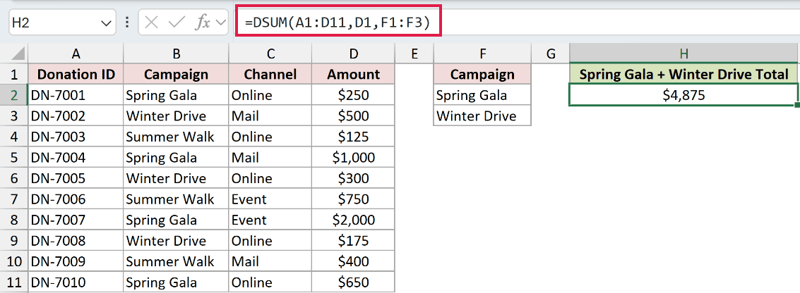
Each campaign occupies its own criteria row, so DSUM treats the rows as OR alternatives. The field argument D1 points to the Amount header.
The combined total is $4,875.
This is where DSUM can be tidier than SUMIFS. Adding another campaign requires another criteria row instead of another function call.
Example 5: Match Partial Text With Wildcards
The hardware list includes Pro in several positions within the model names.
Below is the dataset. Columns A through D contain ten hardware models, with the *Pro* criterion sitting to the right of the list.
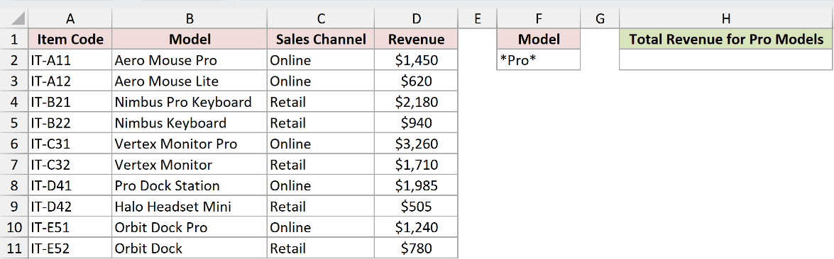
We want to add revenue for every model containing Pro.
Here is the formula:
=DSUM(A1:D11,"Revenue",F1:F2)
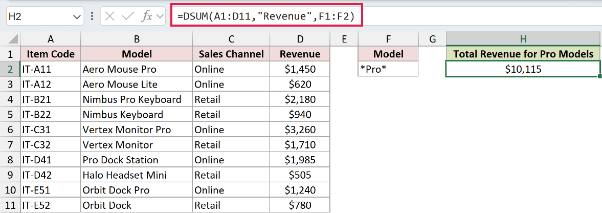
The asterisks allow any characters before or after Pro. Five models match, and DSUM returns $10,115.
Plain Pro would use begins-with matching and return only the Pro Dock Station revenue of $1,985.
Pro Tip: DSUM supports wildcards, but its wildcard behavior is less extensive than SUMIFS. Check a few known records before relying on a wildcard total.
Example 6: Compare DSUM and SUMIFS
A branch-sales sheet lets us compare both formulas against identical records and criteria.
Below is the dataset. Columns A through E hold ten branch sales, while the right-hand criteria panel specifies Lakeview and Flooring.
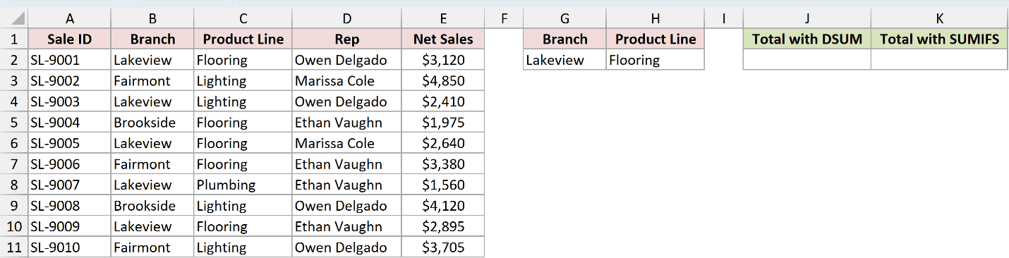
We want to compare DSUM and SUMIFS using the same two conditions.
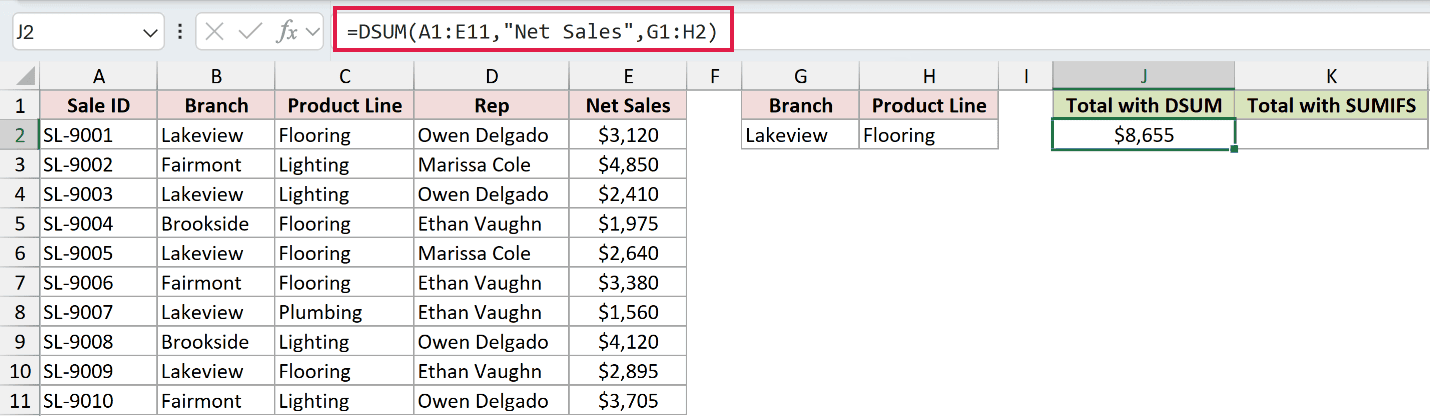
Here is the DSUM formula:
=DSUM(A1:E11,"Net Sales",G1:H2)
And here is the SUMIFS formula for comparison:
=SUMIFS(E2:E11,B2:B11,G2,C2:C11,H2)
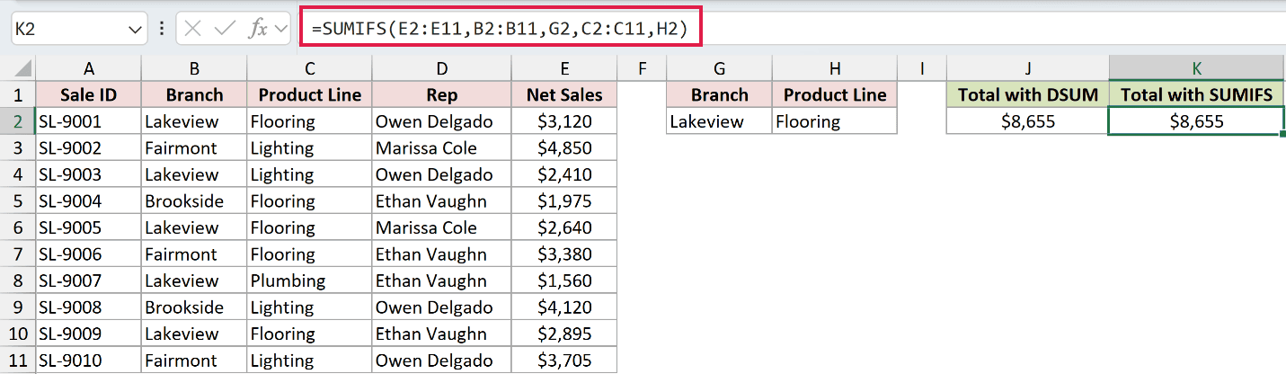
Both formulas return $8,655. DSUM reads the visible criteria block, while SUMIFS places its range relationships inside the formula.
SUMIFS is usually shorter for fixed AND conditions. DSUM is often easier when colleagues need to edit criteria without touching a formula.
In Excel 2021, Excel 2024, and Microsoft 365, SUM with FILTER is the natural dynamic-array alternative. DSUM cannot accept the FILTER result as its database range.
Tips & Common Mistakes
- Include the header row in the database range. Using A2:D11 instead of A1:D11 removes the field names DSUM needs.
- Keep the criteria block beside the list, never below it. New list rows could collide with a criteria range placed underneath.
- Match criteria headers to database headers exactly. A spelling difference or trailing space can cause #VALUE! or an unexpected zero.
- Conditions on the same criteria row use AND logic. Conditions on separate rows use OR logic.
- A blank criteria cell drops that one condition. Clear every cell beneath the criteria headers to return the total for the selected field.
- For Excel Tables, use a range that includes the headers, such as the table’s #All reference. A normal column reference excludes them.
- The same criteria range can also feed DAVERAGE, DCOUNT, DMAX, DMIN, and other database functions.
- Use
=SUM(FILTER(...))for a dynamic-array source. A DSUM formula cannot use a FILTER result as its database argument.
Use Example 1 as a quick reference for a single condition, and Example 4 for OR logic across separate rows.
Once the criteria range is arranged correctly, the same layout also works with the other database functions listed above.
Related Excel Functions / Articles:
Other Excel articles you may also like:
