
Excel’s ARRAYTOTEXT function returns an array as one text string in a single cell. It can create a readable list or text shaped like an Excel array constant.
Blank cells remain as empty items, and number formats are not preserved. ARRAYTOTEXT always returns one cell, so even a strict result does not spill.
In this article, I’ll show you how to compare both formats, reuse strict output as an array constant, and keep dates readable.
ARRAYTOTEXT Function Syntax in Excel
The ARRAYTOTEXT function has the following syntax:
=ARRAYTOTEXT(array, [format])
arrayis the range or array you want to convert to text.[format]is optional. Use 0 for concise format or 1 for strict format. If omitted, it defaults to 0.
When to Use ARRAYTOTEXT Function
- Combine a column or table into one text value for a note, summary, or report.
- Create strict text that you can reuse as a small array constant in another formula.
- Collapse results from FILTER, SORT, or UNIQUE into one cell.
- Inspect the values inside a calculated array in one compact text result.
Example 1: Convert an Array to Text
Let’s start with a basic list.
Below is the dataset with eight discontinued products in column A and an empty One-Line List result cell in C2, ready for the answer.
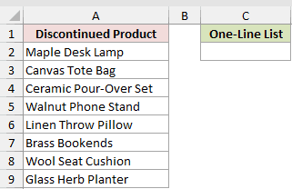
We want to turn the product names into a comma-separated list in one cell.
Here is the formula:
=ARRAYTOTEXT(A2:A9)

Reading A2:A9 from top to bottom, the formula returns all eight product names in C2, separated by a comma and a space.
The function is available in Excel 2021, Excel 2024, and Microsoft 365. It is not available in Excel 2019 or earlier.
Example 2: Compare Concise and Strict Formats
Now let’s compare the two format options.
Below is the dataset with Store, Units Sold, and Open Sundays columns. B3 contains =NA() for Airport, which means not reported yet.
Cells F2 and F3 are waiting for the concise and strict results. Their matching format labels are in E2 and E3.
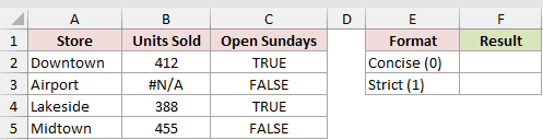
We want to convert A2:C5 using Concise (0) and Strict (1) formats.
Here is the concise formula:
=ARRAYTOTEXT(A2:C5)

And here is the strict formula:
=ARRAYTOTEXT(A2:C5,1)

How these formulas work:
- A2:C5 is read from left to right across each row, then from top to bottom.
- Omitting
formatselects concise format. F2 returnsDowntown, 412, TRUE, Airport, #N/A, FALSE, Lakeside, 388, TRUE, Midtown, 455, FALSE. - Using 1 selects strict format. F3 returns
{"Downtown",412,TRUE;"Airport",#N/A,FALSE;"Lakeside",388,TRUE;"Midtown",455,FALSE}. - Strict format adds braces, quotes text only, uses commas between columns, and uses semicolons between rows in en-US Excel.
- Numbers, TRUE, FALSE, and #N/A are not quoted. The error marker becomes part of the text instead of making ARRAYTOTEXT return an error.
Example 3: Reuse Strict Text as an Array Constant
Here’s a practical reason to use strict format.
Below is the dataset with Zone and Shipping Rate columns in A2:B5. Cell E2 is for the rate table as an array, while E3 is for the Zone 3 rate.
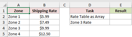
We want to turn the rate table into strict text, then use that text as an array constant in VLOOKUP.
Here is the strict ARRAYTOTEXT formula:
=ARRAYTOTEXT(A2:B5,1)
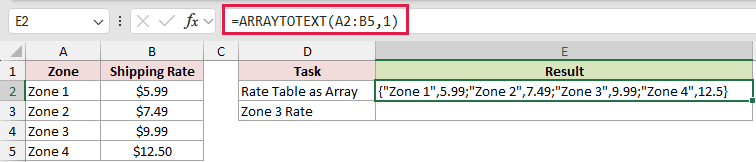
And here is the VLOOKUP formula using that array constant:
=VLOOKUP("Zone 3",{"Zone 1",5.99;"Zone 2",7.49;"Zone 3",9.99;"Zone 4",12.5},2,FALSE)

How these formulas work:
- The first formula returns
{"Zone 1",5.99;"Zone 2",7.49;"Zone 3",9.99;"Zone 4",12.5}in E2. - You can paste that strict string inside VLOOKUP as its table array. VLOOKUP then finds Zone 3 and returns 9.99 in E3.
- Cell formatting is not stored in the text. The source rates show currency, but the constant contains 12.5 rather than $12.50.
Example 4: Keep Dates Readable with TEXT
Dates need a little extra care.
Below is the dataset with Pickup Date values in A2:A6. Cell D2 is for the result without TEXT, while D3 is for the version with TEXT.
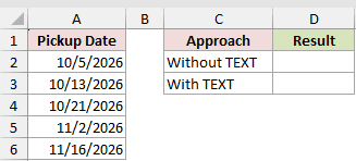
We want to compare the raw date output with dates formatted as short month and day labels.
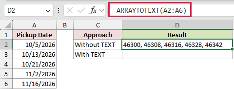
Here is the formula without TEXT:
=ARRAYTOTEXT(A2:A6)
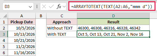
And here is the formula with TEXT:
=ARRAYTOTEXT(TEXT(A2:A6,"mmm d"))
How these formulas work:
- The first formula ignores the date display format and returns
46300, 46308, 46316, 46328, 46342in D2. - TEXT converts each date to the
mmm dpattern before ARRAYTOTEXT joins them. - The second formula returns
Oct 5, Oct 13, Oct 21, Nov 2, Nov 16in D3.
Pro Tip: Apply TEXT before ARRAYTOTEXT whenever displayed dates, currency, percentages, or decimal places must be kept.
Example 5: Combine FILTER Results in One Cell
Let’s use ARRAYTOTEXT with a filtered list.
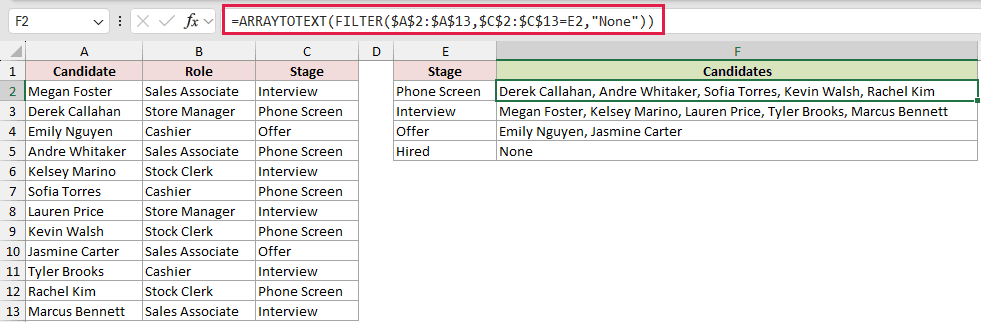
Below is the dataset with Candidate, Role, and Stage columns in A:C. E2:E5 contains the four Stage values, with empty Candidates cells in F2:F5.
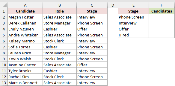
We want one comma-separated candidate list for each hiring stage.
Here is the formula:
=ARRAYTOTEXT(FILTER($A$2:$A$13,$C$2:$C$13=E2,"None"))
How this formula works:
- FILTER returns names from A2:A13 where the Stage in C2:C13 matches E2.
- ARRAYTOTEXT collapses that filtered array into one text value in F2 instead of spilling the names into separate cells.
- For Phone Screen, F2 returns
Derek Callahan, Andre Whitaker, Sofia Torres, Kevin Walsh, Rachel Kim. - Fill the formula through F5. FILTER returns
Nonefor Hired because no candidate has that stage.
Example 6: Create a Sorted Unique List
Here’s another useful array combination.
Below is the dataset with Order ID and Ship-To State columns in A2:B13, with an empty States Shipped To cell in D2.
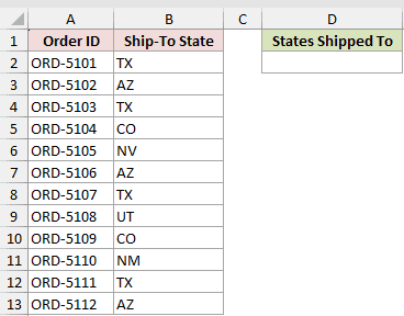
We want one alphabetized text list of the distinct states in the orders.
Here is the formula:
=ARRAYTOTEXT(SORT(UNIQUE(B2:B13)))
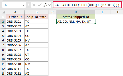
UNIQUE removes repeated state codes from B2:B13, and SORT arranges the remaining codes alphabetically. ARRAYTOTEXT returns AZ, CO, NM, NV, TX, UT in D2.
Example 7: ARRAYTOTEXT vs TEXTJOIN for Blank Cells
Finally, let’s compare how two functions handle blanks.
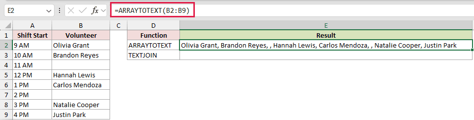
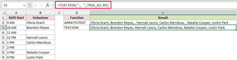
Below is the dataset with Shift Start and Volunteer columns. B4 and B7 are empty, while E2:E3 are empty Result cells for ARRAYTOTEXT and TEXTJOIN.
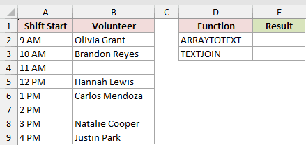
We want to compare a list that keeps the empty volunteer slots with one that skips them.
Here is the ARRAYTOTEXT formula:
=ARRAYTOTEXT(B2:B9)
And here is the TEXTJOIN formula:
=TEXTJOIN(", ",TRUE,B2:B9)
How these formulas work:
- Both empty cells remain as empty items. E2 returns
Olivia Grant, Brandon Reyes, , Hannah Lewis, Carlos Mendoza, , Natalie Cooper, Justin Park. - TEXTJOIN uses TRUE to ignore empty cells. E3 returns
Olivia Grant, Brandon Reyes, Hannah Lewis, Carlos Mendoza, Natalie Cooper, Justin Park. - Concise ARRAYTOTEXT uses its fixed comma and space separator. TEXTJOIN lets you choose the separator and whether empty cells are ignored.
Tips & Common Mistakes
- Only 0 or 1 is accepted for
format. Any other value returns #VALUE!. - Separators follow your Excel locale. The commas and semicolons shown here are for en-US settings and may differ in another region.
- You can wrap ARRAYTOTEXT around an array returned by FILTER, SORT, or UNIQUE to collapse it into one text cell.
- VALUETOTEXT is the single-value counterpart when you need to convert one value rather than an array.
I’ve covered concise and strict output, reusable array constants, readable dates, and ways to combine filtered or unique values in one cell.
I hope you found this article helpful.
Related Excel Functions / Articles:
