
Excel’s AVERAGEA function calculates an average while counting text and logical values in referenced cells. TRUE counts as 1, while FALSE and text count as 0.
Empty cells are ignored, but cells that look blank because a formula returns an empty string still count.
In this article, I’ll show you how text and logical values change an average, calculate rates from TRUE and FALSE entries, and handle formula blanks.
AVERAGEA Function Syntax in Excel
AVERAGEA accepts one required value or reference, followed by up to 254 optional arguments.
=AVERAGEA(value1, [value2], ...)
- value1 (required) is the first value, cell reference, or range you want to average.
- value2, … (optional) are additional values, cell references, or ranges to include.
When to Use AVERAGEA Function
- Treat text entries such as Missing as zero while ignoring truly empty cells.
- Calculate a completion rate from a column of TRUE and FALSE values.
- Find a per-person rate across several logical columns.
- Average spilled TRUE and FALSE flags through a spill reference.
- Include formula-generated empty strings as zero in an average.
Example 1: Average Scores With Missing Work
A gradebook shows the difference clearly when missing work should lower the average.
Below is the dataset. Column B contains scores, two Missing entries, and one empty cell. The labelled cells at the bottom will hold both averages.
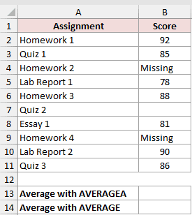
We want an average that counts each Missing entry as zero but skips the empty Quiz 2 cell.
Here is the AVERAGEA formula:
=AVERAGEA(B2:B11)
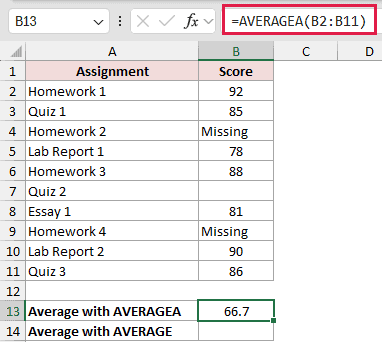
The formula returns 66.7. The two text entries count in the denominator as zeros, while the genuinely empty cell is ignored.
Here is the AVERAGE formula for comparison:
=AVERAGE(B2:B11)
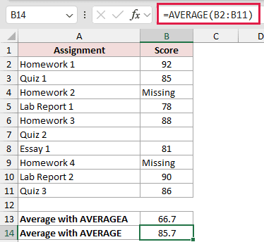
AVERAGE returns 85.7 because it ignores both the Missing entries and the empty cell. That makes it unsuitable when missing work should reduce the grade.
Pro Tip: Leave excused work genuinely empty. Typing a label makes AVERAGEA count that cell as zero.
Example 2: Calculate a Checklist Completion Rate
Here’s a practical way to summarize a TRUE and FALSE checklist.
Below is the dataset. Each employee’s training status appears in column B. The completion-rate cell beneath the list is ready for the formula.
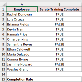
We want one percentage showing how much of the safety training list is complete.
Here is the formula:
=AVERAGEA(B2:B13)
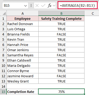
The result is 75%. AVERAGEA treats TRUE as 1 and FALSE as 0, so the average becomes the share of completed entries.
Pro Tip: Microsoft 365 checkboxes store TRUE and FALSE values, so this formula also works with a checkbox column. This workbook uses plain logical values.
Example 3: Find Each Trainee’s Attendance Rate
Attendance records add one wrinkle: the rate belongs to each person.
Below is the dataset. Columns B through F contain five daily attendance values, and column G will hold each trainee’s attendance rate.
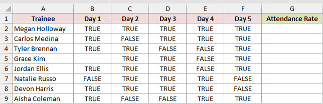
We want to average the logical values across each row, starting with Megan Holloway.
Enter this formula in G2 and copy it down through G9:
=AVERAGEA(B2:F2)
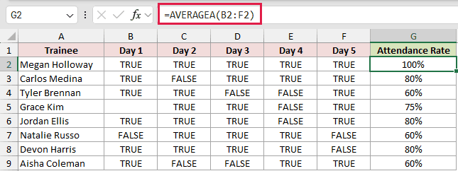
Megan’s row returns 100%. The copied formulas adjust the row references, so every trainee gets a separate result.
Grace Kim’s blank Day 1 cell is ignored, so her row returns 75% instead of treating the unrecorded day as an absence.
Pro Tip: Use FALSE for a recorded absence and leave the cell empty only when that day should not count for the trainee.
Example 4: Average Spilled SLA Flags
Next, we’ll create a visible flag column before averaging it.
Below is the dataset. Column B holds resolution times, with an empty flag column C and an SLA compliance cell waiting below.
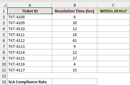
We first want column C to identify tickets resolved within 24 hours.
Here is the spilling formula in C2:
=B2:B11<=24
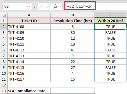
The comparison spills TRUE and FALSE results through C11. The visible helper column also makes it easy to spot tickets that missed the target.
We can then average the entire spill through the spill range reference C2#.
Here is the formula:
=AVERAGEA(C2#)
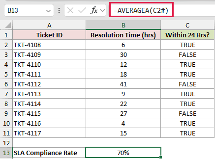
The result is 70%. The hash sign tells Excel to use every logical value produced by the spill that starts in C2.
The spill and the C2# reference require Excel 2021, Excel 2024, or Microsoft 365.
Pro Tip: Keep the comparison in a helper column. AVERAGEA ignores logicals created inside a computed array, so =AVERAGEA(B2:B11<=24) returns #DIV/0!. The spill range reference C2# points to worksheet cells instead.
Example 5: Handle Formula Blanks Correctly
Formula blanks need a closer look because they are not empty cells.
Below is the dataset. Column B counts responses, while column C counts satisfied responses. Column D and the two comparison cells beneath the table are ready for results.
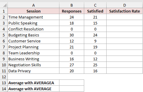
We first want each session’s satisfaction rate while hiding division errors for sessions with no responses.
Enter this formula in D2 and copy it down through D11:
=IF(B2=0,"",C2/B2)
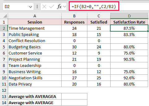
The formulas in D4 and D8 return empty strings. Those cells look blank, but AVERAGEA still treats each one as a zero.
Here is the AVERAGEA formula:
=AVERAGEA(D2:D11)
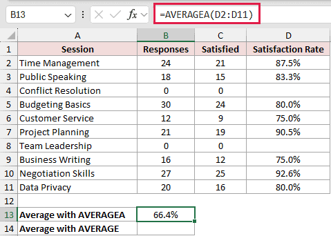
AVERAGEA returns 66.4% because both empty strings stay in its denominator as zeros.
Here is the AVERAGE formula for comparison:
=AVERAGE(D2:D11)
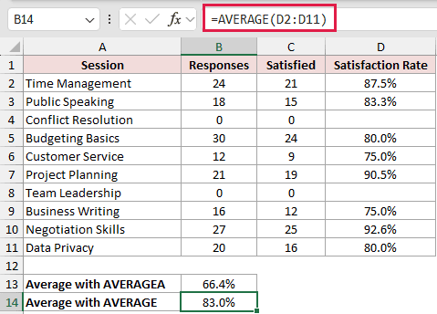
AVERAGE ignores the empty strings and returns 83.0%. Use that version when sessions with no responses should not affect the average.
Pro Tip: A formula-generated empty string is not the same as an unused cell. Check the underlying formula when blank-looking cells pull an AVERAGEA result down.
Tips & Common Mistakes
- AVERAGEA returns one result from a range. It does not spill an average for every row or column on its own.
- In references, every non-empty cell that COUNTA counts joins the denominator. Numbers contribute their value, TRUE contributes 1, while FALSE and text contribute 0.
- A number stored as text contributes 0 in a referenced cell. Convert it to a real number before using AVERAGEA when its numeric value should count.
- Yes and No text entries do not behave like TRUE and FALSE. Use real logical values when you want a completion percentage.
- Use AVERAGE when you want a numbers-only result or need formula-generated empty strings excluded.
- Errors in a referenced range pass through to the result. Fix or handle those errors before calculating the average.
- Logical values typed directly into the argument list count, so
=AVERAGEA(TRUE,FALSE,5)returns 2. Typed nonnumeric text causes an error, so=AVERAGEA(5,"abc")returns#VALUE!.
AVERAGEA is dependable when the source range reflects your scoring rules.
Define what should count as zero before entering text or FALSE into that range.
Related Excel Functions / Articles:
