
Excel’s HOUR function returns the hour portion of a time or date-time as an integer from 0 to 23.
It reads the clock hour, not elapsed time. Minutes are dropped without rounding, so 7:59 AM returns 7 and 12:05 AM returns 0.
In this article, I’ll show you how to extract hours, label shifts, count and filter records by hour, and handle durations longer than 24 hours.
HOUR Function Syntax in Excel
The HOUR function uses the following syntax:
=HOUR(serial_number)
- serial_number: Required. A valid Excel time, date-time, text time, or formula result containing a time.
When to Use HOUR Function
- Extract the hour from time stamps for reporting or grouping.
- Convert mixed text times into consistent hour numbers.
- Assign records to shifts or other time-of-day categories.
- Count or filter transactions that fall within selected hours.
- Check the clock-hour portion of a time difference.
Example 1: Extract Hour From Date-Time
Let’s start with a simple pickup log.
Below is the dataset with trip IDs, pickup date-times, and an empty Pickup Hour column waiting for the results.
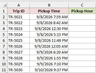
We want to return the pickup hour for every trip in column C.
Here is the formula:
=HOUR(B2:B11)
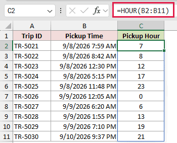
The formula reads each date-time in B2:B11 and returns only its hour. The Power Query counterpart can do this during data preparation.
The date, minutes, and seconds do not appear in the result. The TIME function can rebuild a time with chosen minutes and seconds.
For example, 7:59 AM returns 7, 11:48 PM returns 23, and 12:05 AM returns 0.
Pro Tip: This range formula spills automatically in Excel 2021, Excel 2024, and Microsoft 365. In Excel 2019 and earlier, use one formula per row.
Example 2: Convert Text Times to Hours
Imported booking data often stores requested times as text.
Below is the dataset with booking references, requested slots stored as text, and an empty Slot Hour column waiting for the results.
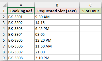
We want to convert each text time into its hour number.
Here is the formula:
=HOUR(B2:B9)
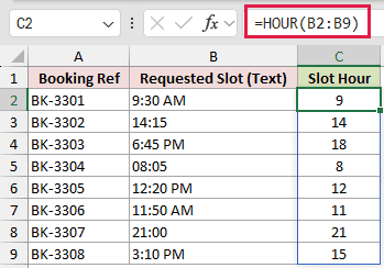
HOUR converts recognized text times itself, so a TIMEVALUE wrapper is unnecessary. It always returns the answer on the 24-hour clock.
That means 14:15 returns 14, 3:10 PM returns 15, and 12:20 PM returns 12.
Example 3: Assign Work Shifts by Hour
Now let’s use the extracted hour to label warehouse shifts.
Below is the dataset with pick IDs, scan date-times, and an empty Shift column waiting for the assigned labels.
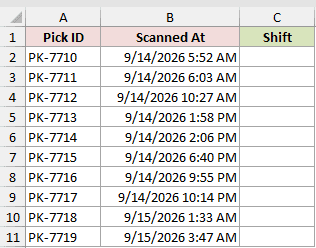
We want to assign First, Second, or Third shift from each scan time.
Here is the formula:
=IFS(HOUR(B2:B11)<6,"Third",HOUR(B2:B11)<14,"First",HOUR(B2:B11)<22,"Second",TRUE,"Third")
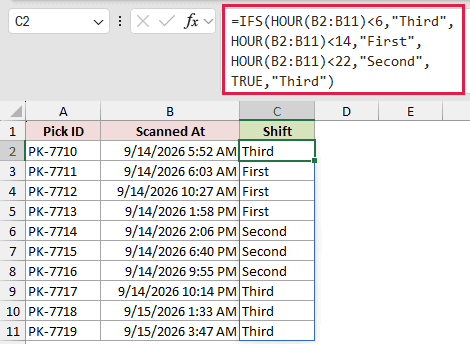
IFS is available in Microsoft 365, Excel 2024, Excel 2021, and Excel 2019.
How this formula works:
HOUR(B2:B11)returns the hour for each scan time.- IFS checks its tests in order. Hours 0 to 5 are assigned Third, and hours 6 to 13 are assigned First.
- Hours 14 to 21 are assigned Second. The final
TRUEsends hours 22 to 23 to Third.
The first test and final fallback cover the overnight shift together. For example, 10:14 PM and 1:33 AM both return Third.
Pro Tip: LET is available in Microsoft 365, Excel 2024, and Excel 2021. It can calculate the hour once with =LET(h,HOUR(B2:B11),IFS(h<6,"Third",h<14,"First",h<22,"Second",TRUE,"Third")). The original formula still works and keeps each boundary visible.
Example 4: Count Entries by Hour
We can count entries in this parking log to find its busiest arrival periods.
Below is the dataset with parking tickets, entry date-times, hours 6 through 11, and an empty Cars In column waiting for the counts.
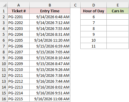
We want to count how many cars entered during each listed hour across all dates.
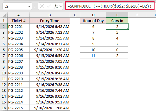
Here is the formula:
=SUMPRODUCT(--(HOUR($B$2:$B$16)=D2))
How this formula works:
HOUR($B$2:$B$16)returns an array of entry hours from the fixed date-time range.- Comparing that array with
D2identifies entries that occurred during the listed hour. - The double unary converts TRUE and FALSE values to 1 and 0, then SUMPRODUCT adds the matches.
The formula returns 2 for hour 6. Fill it from E2 through E7 to return 2, 5, 4, 2, 0, and 2.
We keep this calculation per row because COUNTIF cannot use HOUR(range) as its range. The fixed hour list also keeps hour 10 visible with a zero count.
Example 5: Filter Orders by Hour Range
Next, let’s pull every order placed during the lunch rush.
Below is the dataset with order details on the left and a matching empty result area on the right waiting for the filtered rows.
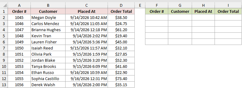
We want to return orders placed from 11:00 AM up to, but not including, 2:00 PM.
Here is the formula:
=FILTER(A2:D13,(HOUR(C2:C13)>=11)*(HOUR(C2:C13)<14))
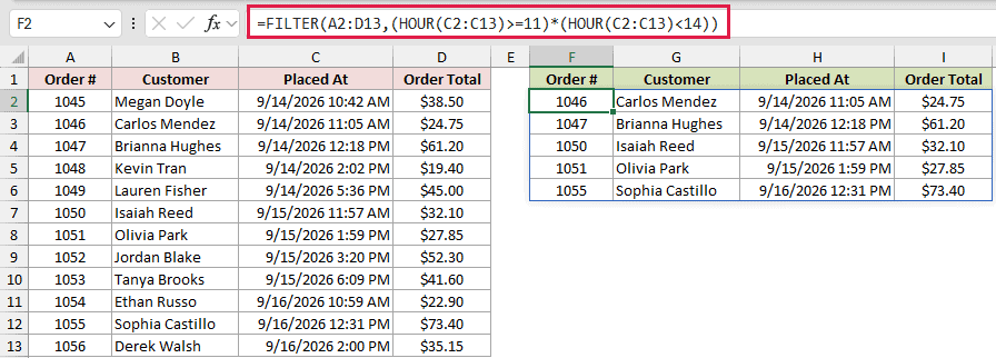
How this formula works:
HOUR(C2:C13)>=11keeps orders at 11:00 AM or later.HOUR(C2:C13)<14keeps orders before 2:00 PM.- Multiplying the two tests makes FILTER return only rows where both conditions are TRUE.
The formula returns orders 1046, 1047, 1050, 1051, and 1055.
The 10:59 AM order is dropped, the 1:59 PM order is kept, and the order at exactly 2:00 PM is dropped.
FILTER is available in Microsoft 365, Excel 2024, and Excel 2021.
Example 6: Calculate Hours Over 24 Hours
Finally, let’s compare clock hours with true elapsed hours.
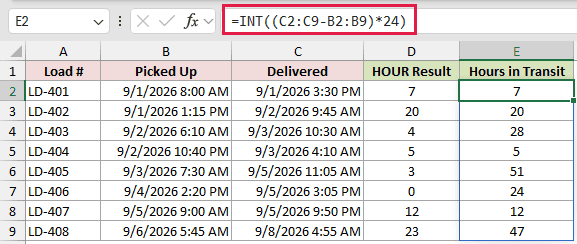
Below is the dataset with load numbers, pickup and delivery date-times, and empty HOUR Result and Hours in Transit columns waiting for answers.
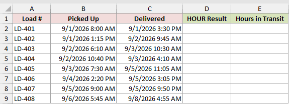
We want to compare HOUR’s clock reading with the number of complete hours each delivery took.
Here is the formula:
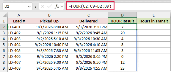
=HOUR(C2:C9-B2:B9)
For the true full-hour count, use this formula:
=INT((C2:C9-B2:B9)*24)
How these formulas work:
- Subtracting pickup from delivery returns elapsed time as a fraction of a day.
- HOUR reads only the clock-hour portion and resets every 24 hours. A duration of 28 hours 20 minutes therefore returns 4.
- Multiplying the difference by 24 converts it to hours. INT removes the remaining fraction, so 28 hours 20 minutes returns 28 full hours.
The first row returns 7 with both formulas. Longer trips expose the difference, including 51 hours 35 minutes, which returns 3 with HOUR and 51 with INT.
Tips & Common Mistakes
- HOUR returns a clock reading from 0 to 23, not a duration. Use the full date-time difference when elapsed time can cross midnight or exceed 24 hours.
- HOUR drops minutes without rounding. A time of 12:05 AM returns 0, not 1.
HOUR(8.5)returns 12, not 8. Excel treats 8.5 as eight days plus half a day, so HOUR reads noon from the fractional part. For a time in B2,=HOUR(B2)+MINUTE(B2)/60can convert time to decimal hours.- A date with no time returns 0 because its time portion is midnight.
- To keep the date and bucket a stamp into its hour, the FLOOR function formula
FLOOR(B2,"1:00")rounds the stamp down. - The NOW function inside
HOUR(NOW())returns the current hour of the day. - In Excel 2021, Excel 2024, and Microsoft 365, HOUR range formulas spill into neighboring cells. Blocked output cells cause a
#SPILL!error. - For Examples 1, 2, and 6, Excel 2019 and earlier need one formula per row. An implicit-intersection
@reduces a range result to one cell. - Unrecognized text times can return
#VALUE!. Negative or otherwise out-of-range time values can return#NUM!.
I’ve covered extracting clock hours from date-times and text, then using those results to group records and check longer time differences.
I hope you found this article helpful.
Related Excel Functions / Articles:
