
The MINUTE function in Excel returns the minute part of a time as a whole number from 0 to 59.
You can use that number to check scheduled departures or separate the minutes from a timestamp. The date and hour don’t become part of the result.
For durations, MINUTE returns only the minute component, so it doesn’t tell you the total time spent on a task.
In this article, I’ll show you how to extract minutes from timestamps and text, calculate session totals, and bill rentals in quarter-hour blocks.
MINUTE Function Syntax in Excel
MINUTE takes the time value you want to read:
=MINUTE(serial_number)
- serial_number (required) is a time, date-time, or recognizable text time. You can supply a cell reference or a range of cells.
Excel stores times as fractions of a day. MINUTE reads the minutes from that stored value and returns a number you can use in other calculations.
When to Use MINUTE Function
- Extract the minute component from a column of timestamps.
- Read the minutes from imported text times Excel recognizes.
- Combine minutes with hours to calculate short session durations.
- Round rental durations up to billing increments.
- Check whether departures follow an hourly or half-hourly schedule.
Example 1: Extract Minutes From Date-Times
Let’s start with an office badge-swipe log that includes dates, times, and seconds.
Below is the dataset. Column A lists badge numbers, column B holds swipe timestamps, and column C has the Minute header ready for the results.
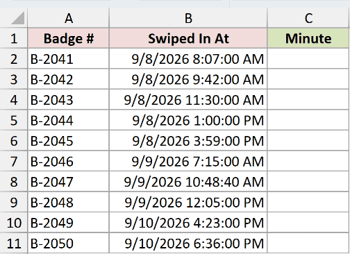
We want to extract the minute from each timestamp without changing the original log.
Enter this formula in C2:
=MINUTE(B2:B11)
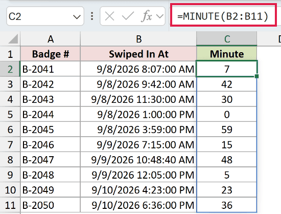
The formula spills into C2:C11, returning a minute for each timestamp in B2:B11.
Range formulas spill in Excel 2021, Excel 2024, and Microsoft 365. In Excel 2019 and earlier, reference each row’s time individually and fill down.
Badge B-2041 has the timestamp 9/8/2026 8:07:00 AM, so its result is 7. Badge B-2044 returns 0 from 9/8/2026 1:00:00 PM.
Badge B-2047 returns 48 from 9/9/2026 10:48:40 AM. The 40 seconds are dropped rather than rounded up to the next minute.
Pro Tip: Keep the output cells below C2 empty before entering the formula. A blocked spill range produces #SPILL!.
Example 2: Pull Minutes From Text Times
Imported class schedules don’t always arrive as numeric Excel times.
Below is the dataset. Column A lists classes, column B contains text times and a TBD entry, and column C is reserved for Start Minute.
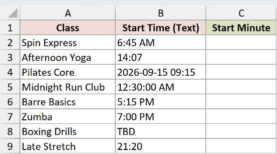
We want to read the minutes from these text entries and see which entry Excel can’t interpret.
Enter this formula in C2:
=MINUTE(B2:B9)
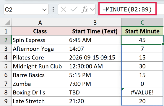
The results spill into C2:C9.
TIMEVALUE turns a text time into an Excel time value, but MINUTE handles that conversion itself, so these entries don’t need it.
Spin Express returns 45 from 6:45 AM, while Afternoon Yoga returns 7 from 14:07.
The date-time text 2026-09-15 09:15 returns 15 for Pilates Core. Midnight Run Club’s 12:30:00 AM returns 30.
Boxing Drills deliberately contains TBD, so C8 shows #VALUE!.
Replace TBD with the actual start time when it’s known. Hiding the error with a zero would make an unknown start look like an on-the-hour class.
Example 3: Minute Part Versus Total Minutes
A studio session makes the difference between a minute component and elapsed minutes easier to see.
Below is the dataset. Columns B and C hold session start and end times; D holds the minute-part comparison, and E is reserved for Total Minutes.
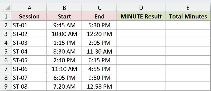
We want total session lengths, and we’ll first show why MINUTE alone is the wrong calculation for that job.
Enter this deliberate minute-part comparison in D2:
=MINUTE(C2:C9-B2:B9)
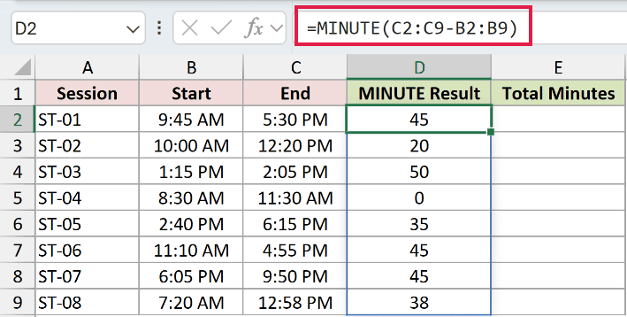
The comparison spills into D2:D9. It subtracts each start from its end, but MINUTE then keeps only the minute part of that duration.
For ST-01, the comparison returns 45 even though the session runs from 9:45 AM to 5:30 PM. Treating 45 as the total would lose the hours.
To include the hours, enter this formula in E2:
=HOUR(C2:C9-B2:B9)*60+MINUTE(C2:C9-B2:B9)
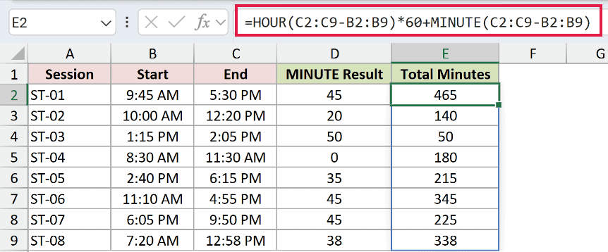
This formula spills the totals into E2:E9. HOUR extracts the hours, multiplication by 60 converts them to minutes, and MINUTE adds the remaining minute component.
ST-01 now returns 465 total minutes. ST-04 returns 180, while its misleading minute-part comparison shows 0 because the session ends on the same minute it started.
Pro Tip: This calculation fits these same-day sessions, which last less than 24 hours. HOUR wraps at a day, so use a full elapsed-time calculation for longer durations.
Example 4: Bill Rentals in 15-Minute Blocks
Now let’s use the minute component to round kayak rentals up to the next billing block.
Below is the dataset. Columns B and C record Out and Back times, with Duration and Billed Minutes headers in columns D and E.
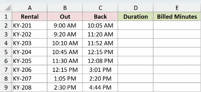
We want each rental’s duration, followed by its billed minutes rounded up to a 15-minute increment.
First, enter the duration formula in D2:
=C2:C9-B2:B9
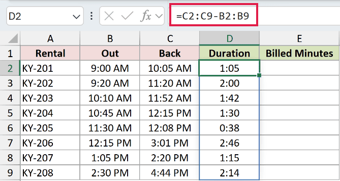
The durations spill into D2:D9, formatted as h:mm. KY-201 displays 1:05, and KY-203 displays 1:42.
Next, enter the billing formula in E2:
=HOUR(D2:D9)*60+CEILING(MINUTE(D2:D9),15)
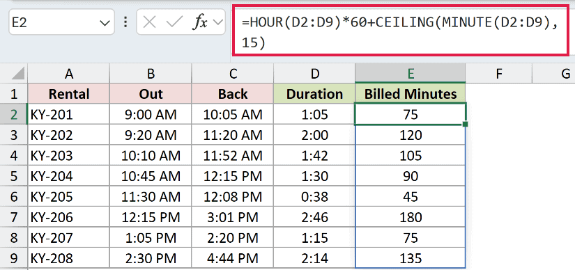
The billed minutes spill into E2:E9.
How this formula works:
- HOUR reads the whole-hour component of each duration, and multiplying by 60 converts it to minutes.
- MINUTE reads the remaining minute component.
- CEILING rounds that component up to a multiple of 15 before the formula adds it to the whole-hour minutes.
KY-201’s 1:05 duration bills as 75 minutes. KY-203’s 1:42 bills as 105 minutes.
KY-204’s 1:30 already falls on a billing boundary and stays at 90 minutes. KY-206’s 2:46 rounds up to 180 billed minutes.
Pro Tip: These rental times are recorded to whole minutes and stay within the same day. Don’t use this formula unchanged for multi-day rentals or a billing policy that charges for partial minutes.
Example 5: Check Half-Hourly Departures
MINUTE can also supply the number a schedule check needs.
Below is the dataset. Column A lists trips, column B contains departure times, and column C has the Timetable Check header ready for the labels.
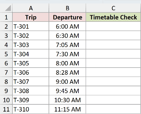
We want to flag departures that aren’t on the hour or half-hour.
Enter this formula in C2:
=IF(MOD(MINUTE(B2:B11),30)=0,"On Timetable","Check")
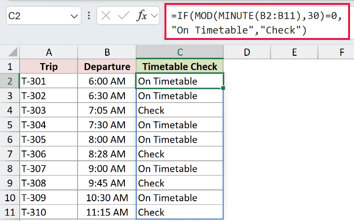
The labels spill into C2:C11. MINUTE extracts each departure’s minute, and MOD checks the remainder after dividing that number by 30.
Minutes of 0 or 30 leave a remainder of 0. IF labels those departures On Timetable and labels the others Check.
T-301 at 6:00 AM and T-302 at 6:30 AM return On Timetable. T-303 at 7:05 AM and T-306 at 8:28 AM return Check.
This checks the minute position within the hour. You’ll need separate checks for each trip’s assigned hour and any missing departures.
Tips & Common Mistakes
- A blank can look like a valid minute. MINUTE returns 0 for a truly empty referenced cell. Check missing inputs before interpreting that result as an on-the-hour time.
- Empty text is different from a blank cell. An empty string returns
#VALUE!, as does text Excel can’t recognize as a time. - Fractional seconds can roll into the next minute. In testing, the text time
9:59:59.4returned 59, but9:59:59.5returned 0 because Excel rounded to the next second first. - Negative serials fail. A negative time value returns
#NUM!. With time-only start and end cells, check whether an end before its start represents an overnight session. - Numeric inputs represent days. An input of 1.1 returns 24 because its fractional day represents
2:24. A plain number isn’t interpreted as a count of minutes. Use TIME to build a time from separate hour, minute, and second values. - MINUTE returns a component. Use HOUR alongside it when hours belong in a short-duration total, as shown in the studio and rental examples.
Related Excel Functions / Articles:
