
Excel’s MODE.MULT function returns a vertical array of every numeric value tied for the highest frequency in a dataset.
MODE.MULT is especially useful when mean, median, and mode comparisons reveal more than one mode. MODE.SNGL returns only the tied mode that appears first.
The examples count tied modes, handle unique data, calculate modes by group, and find the most common text values.
MODE.MULT Function Syntax in Excel
The MODE.MULT function uses the following syntax:
=MODE.MULT(number1, [number2], ...)
number1: The first number, array, or cell reference you want to evaluate.number2: Optional. Additional numbers, arrays, or references. MODE.MULT accepts up to 254 number arguments.
When to Use MODE.MULT Function
- Find every size, score, price, or quantity tied as the most common value.
- Keep all tied modes instead of returning only one with MODE.SNGL.
- Count how often each mode occurs or how many values share the highest frequency.
- Find modes within categories or return modes horizontally for a compact report.
- Identify the most common text values after converting them to numeric positions.
Example 1: Return All Tied Modes
Let’s start with a simple tie.
Below is the dataset of order numbers, shoe styles, and sizes in A1:C15. The empty Most Common Size cells in E2:E3 are waiting for the results.
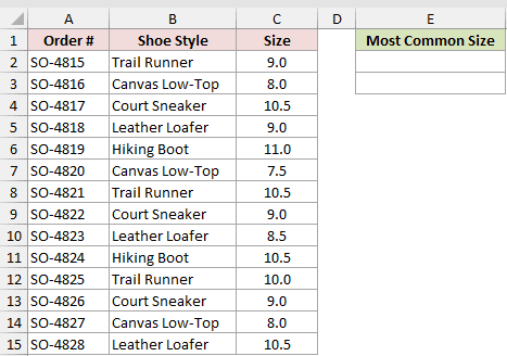
We want to return every shoe size tied as the most common size.
Here is the formula:
=MODE.MULT(C2:C15)
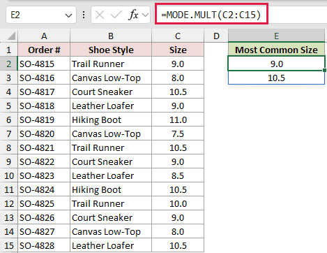
MODE.MULT checks C2:C15 and finds that 9.0 and 10.5 each appear four times. Both values spill vertically into E2:E3.
Pro Tip: In Excel 2021, Excel 2024, and Microsoft 365, enter the formula in E2 and leave E3 clear. In Excel 2019 and earlier, select E2:E3 first and press Ctrl+Shift+Enter.
Example 2: MODE.MULT vs MODE.SNGL in Excel
This example shows what MODE.SNGL leaves out when two values tie.
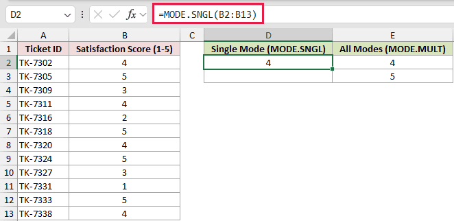
Below is the dataset of ticket IDs and Satisfaction Score (1-5) values in A1:B13. Single Mode (MODE.SNGL) in D2 and All Modes (MODE.MULT) in E2:E3 are empty.
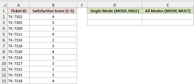
We want to compare the complete set of modes with the single value returned by MODE.SNGL.
Here is the formula:
=MODE.MULT(B2:B13)
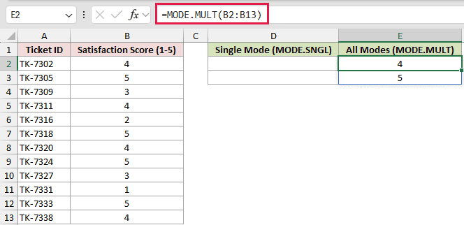
For comparison, here is the MODE.SNGL formula:
=MODE.SNGL(B2:B13)
How these formulas work:
- MODE.MULT returns 4 and 5 because each score appears four times.
- MODE.SNGL returns only 4, the tied mode that appears first in the list.
Example 3: Count Each Mode and the Ties
Let’s add frequency information to the result.
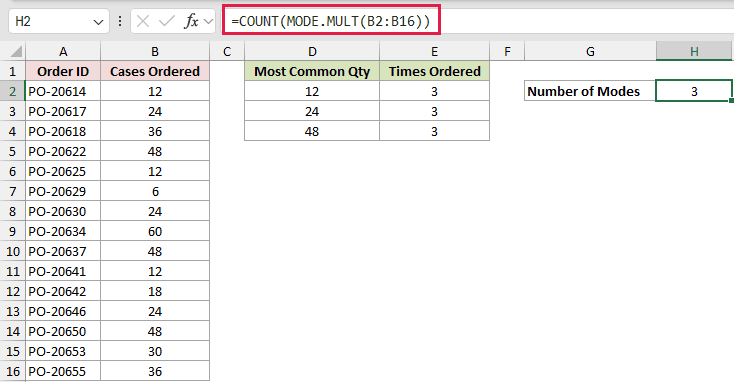
Below is the dataset of order IDs and Cases Ordered in A1:B16. Most Common Qty in D2:D4 and Times Ordered in E2:E4 are empty.
Number of Modes is labelled in G2, with its empty result in H2.
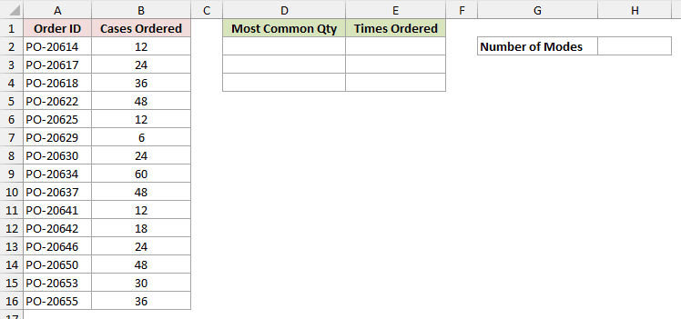
We want to list the tied quantities, count their occurrences, and count how many modes share the highest frequency.
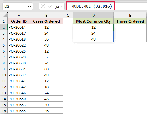
Here is the formula for the most common quantities:
=MODE.MULT(B2:B16)
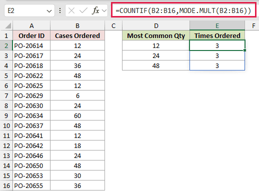
Here is the formula for the number of times each mode was ordered:
=COUNTIF(B2:B16,MODE.MULT(B2:B16))
Here is the formula for the number of modes:
=COUNT(MODE.MULT(B2:B16))
How these formulas work:
- MODE.MULT returns 12, 24, and 48 in D2:D4.
- COUNTIF uses those returned values as criteria and returns 3 beside each one in E2:E4.
- COUNT returns 3 in H2 because three quantities are tied as modes.
Example 4: Handle #N/A When Nothing Repeats
Now let’s see what happens when every value is unique.
Below is the dataset of listing IDs and Sale Price values in A1:B11. The Most Common Price and With IFNA result cells in D2 and E2 are empty.
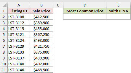
We want to see the default result, then replace it with a clear message for the reader.
Here is the basic formula:
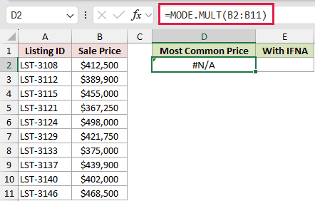
=MODE.MULT(B2:B11)
Here is the formula with IFNA:
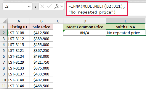
=IFNA(MODE.MULT(B2:B11),"No repeated price")
How these formulas work:
- MODE.MULT returns #N/A because none of the prices repeats.
- IFNA catches that specific error and returns No repeated price in E2.
Pro Tip: Use IFNA instead of IFERROR here. Other error types, such as #DIV/0!, still show, but a #N/A already in the data also becomes the message.
Example 5: Return MODE.MULT Results Horizontally
Here’s a compact layout for a dashboard or summary.
Below is the dataset of delivery IDs and Delivery Time (min) values in A1:B13. The Most Common Times (min) card has two empty result cells in E2:F2.
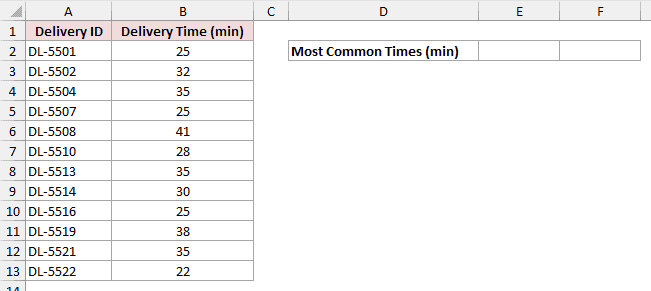
We want to return the tied delivery times across one row instead of down a column.
Here is the formula:
=TRANSPOSE(MODE.MULT(B2:B13))
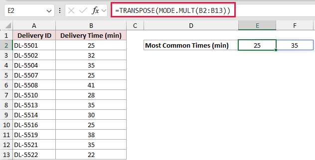
MODE.MULT returns 25 and 35 because each appears three times. TRANSPOSE rotates that vertical array, so the values spill horizontally into E2:F2.
Pro Tip: Leave the cells to the right of E2 empty so the transposed result has room to spill.
Example 6: Find the Mode by Group
Let’s calculate a separate mode for each location.
Below is the reservation dataset in A1:C16. Locations appear again in E2:E4, and the Most Common Party Size cells in F2:F4 are empty.
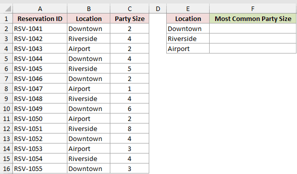
We want to return the most common party size for each location while keeping any ties in one cell.
Here is the formula:
=TEXTJOIN(", ",TRUE,MODE.MULT(FILTER($C$2:$C$16,$B$2:$B$16=E2)))
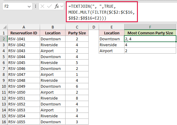
How this formula works:
- FILTER keeps the party sizes for the location in E2.
- MODE.MULT returns every tied mode from that filtered list.
- TEXTJOIN combines multiple modes with a comma and space, so Downtown returns 2, 4 in F2.
- The formula is filled through F4. Riverside returns 4, and Airport returns 2.
Pro Tip: This example requires Excel 2021, Excel 2024, or Microsoft 365 because it uses FILTER.
Example 7: Find the Most Common Text Values
MODE.MULT ignores text, so this formula converts text values to numeric positions before finding the modes.
Below is the dataset of order numbers and Shirt Color values in A1:B15. The two Most Common Color cells in D2:D3 are empty.
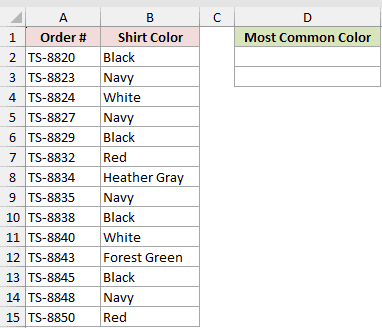
We want to return every shirt color tied as the most common text value.
Here is the formula:
=INDEX(B2:B15,MODE.MULT(MATCH(B2:B15,B2:B15,0)))
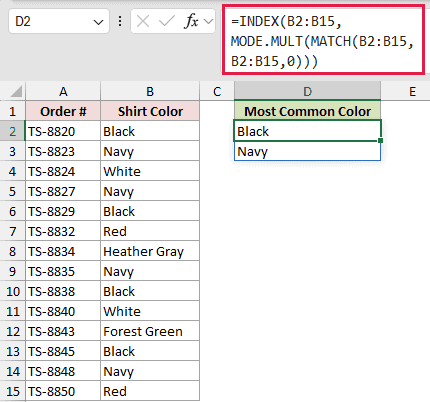
How this formula works:
- MATCH converts each color to the position of its first occurrence in B2:B15.
- MODE.MULT finds the positions that occur most often.
- INDEX returns the corresponding colors, Black and Navy, in D2:D3.
In Excel 2021 and later, the UNIQUE function supports a direct text approach: =LET(u,UNIQUE(B2:B15),c,COUNTIF(B2:B15,u),FILTER(u,c=MAX(c))).
The INDEX and MATCH formula remains useful in Excel versions without LET, UNIQUE, and FILTER.
Pro Tip: The MATCH technique needs a source range with no blank cells.
Tips & Common Mistakes
- Tied modes return in the order they first appear in the data, not in sorted order. Wrap MODE.MULT in SORT when you need a guaranteed order.
- Keep the spill area clear. Occupied cells below the anchor, or to the right of a TRANSPOSE result, can cause a #SPILL! error.
- MODE.SNGL returns only the first mode to appear. It does not necessarily return the lowest mode.
- Text, logical values, and empty cells inside references are ignored. Zeros count, and error values in the data return an error.
- Clean source errors before adding IFNA. A source #N/A and the no-mode #N/A produce the same message, while errors such as #DIV/0! still show.
- In Power Query, List.Modes returns every tied mode while the data is being prepared for the worksheet.
I’ve covered how MODE.MULT returns every tied numeric mode in a spill range.
I hope you found this article helpful.
Related Excel Functions / Articles:
