
Excel’s FACTDOUBLE function returns the double factorial of a number. It multiplies that number by every second positive integer below it.
For example, the double factorial of 7 is 7 × 5 × 3 × 1, or 105. The two exclamation marks in 7!! describe this pattern.
I’ll show you how odd and even inputs work, calculate a whole column, and count ways to pair people into partners.
FACTDOUBLE Function Syntax in Excel
FACTDOUBLE takes one required argument:
=FACTDOUBLE(number)
- number: The nonnegative number whose double factorial you want. You can enter a number or reference a cell. Decimal inputs are truncated to integers.
When to Use FACTDOUBLE Function
- Multiply a sequence of positive integers that decreases by two.
- Calculate double factorials for a list of numbers.
- Count the ways to split an even-sized group into pairs.
- Compare double factorials with ordinary factorials in a mathematical worksheet.
Example 1: Calculate Odd and Even Double Factorials
Let’s start by seeing exactly which numbers get multiplied.
Below is the dataset with Number and Multiplied Out columns, plus empty result cells under Double Factorial.
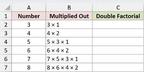
We want to calculate each number’s double factorial in C2:C7.
Here is the formula:
=FACTDOUBLE(A2)
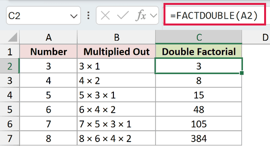
Enter the formula in C2, then fill it down to C7. Each copied formula uses the number in its own row.
The first result is 3 because 3 × 1 equals 3. For the next row, 4 × 2 returns 8.
Odd inputs continue down to 1. The value 7 in A6 produces 7 × 5 × 3 × 1, returning 105 in C6.
Even inputs continue down to 2. The value 8 in A7 produces 8 × 6 × 4 × 2, returning 384 in C7.
Pro Tip: We’re using individual cell references here to match each result to its multiplication pattern. The next example shows how to calculate the whole list with one formula.
Example 2: Calculate a Whole Column
A range needs one small adjustment before FACTDOUBLE can return multiple results.
Below is the dataset with numbers in A2:A7, empty Double Factorial cells, and a separate Bare Range (No Plus Sign) comparison row.
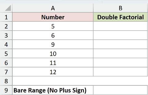
We want one formula in B2 to calculate double factorials for all six numbers.
Here is the formula:
=FACTDOUBLE(+A2:A7)
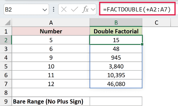
The plus sign converts the range reference into an array of values. FACTDOUBLE processes those values, and the results spill from B2 through B7.
The inputs 5, 6, 9, 10, 11, and 12 return 15, 48, 945, 3,840, 10,395, and 46,080, respectively.
Now enter the comparison formula in B9:
=FACTDOUBLE(A2:A7)
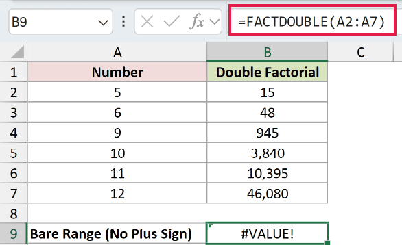
This returns a single #VALUE! error. The numbers are valid, but FACTDOUBLE does not process this bare range reference the same way as the converted array.
Pro Tip: These spill examples use dynamic arrays, available in Excel 2021, Excel 2024, and Microsoft 365. Keep the output cells empty. In Excel 2019 and earlier, use individual cell references and fill down, as in Example 1.
Example 3: Count Ways to Pair People
This example counts the different ways to divide everyone in a team into pairs.
Below is the dataset with Team and Attendees columns, plus empty Ways to Pair Up cells in C2:C7.
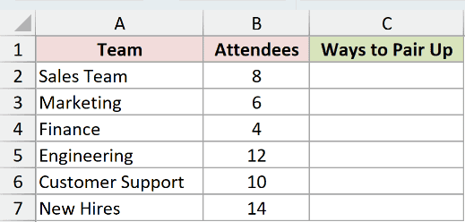
We want to count all possible pairings within each team, with every attendee assigned exactly one partner.
Here is the formula:
=FACTDOUBLE(B2:B7-1)
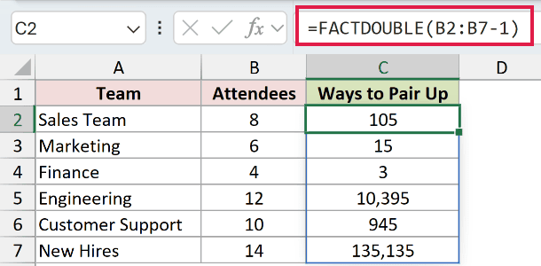
Enter the formula in C2. It spills the pairing counts through C7.
How this formula works:
B2:B7-1subtracts one from each attendance count. The Sales Team’s 8 attendees become an input of 7.- Choose one person first. They have 7 possible partners. Once that pair is formed, the next unpaired person has 5 possible partners, then 3, then 1.
- FACTDOUBLE multiplies those choices: 7 × 5 × 3 × 1 equals 105 possible pairings for the Sales Team.
- Subtracting one already creates an array of values, so this formula does not need the extra plus sign from Example 2.
Marketing’s 6 attendees have 15 possible pairings, while Finance’s 4 attendees have 3. The 14 New Hires have 135,135 possible pairings.
Pro Tip: This count assumes an even number of distinct people, with anyone allowed to partner with anyone else. Pair order and partner order do not matter.
Example 4: Compare FACTDOUBLE with FACT
An ordinary factorial includes every positive integer up to the input, while a double factorial includes every other one.
Below is the dataset with Number (n) values from 3 to 8 and empty columns for both double factorials, their product, and FACT(n).
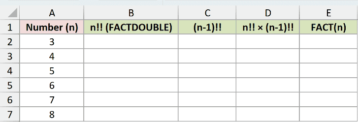
We want to check that multiplying n!! by (n-1)!! produces the same result as n!.
Here is the formula:
=FACTDOUBLE(+A2:A7)
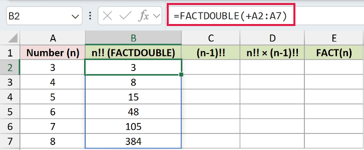
Enter this in B2, and the results spill to B7. For n = 6, the result in B5 is 48, calculated as 6 × 4 × 2.
Next, enter this formula in C2 to calculate the double factorial of each number minus one:
=FACTDOUBLE(A2:A7-1)
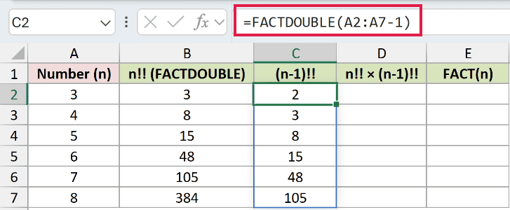
For that same row, C5 returns 15 from 5 × 3 × 1. Together, the two calculations contain every integer from 1 through 6.
Column D uses =B2:B7*C2:C7 in D2 to multiply each row’s double factorials, so D5 returns 48 × 15 = 720.
Column E uses =FACT(A2:A7) in E2 to calculate the ordinary factorials for comparison.
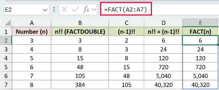
Columns D and E match throughout: 6, 24, 120, 720, 5,040, and 40,320.
Pro Tip: A double factorial does not mean applying FACT twice. Use FACT when you need every integer multiplied together. Use FACTDOUBLE when the sequence steps by two.
Example 5: Check Decimal Inputs and Errors
Let’s finish by checking inputs that can produce unexpected results.
Below is the dataset with Input values, empty FACTDOUBLE Result cells, and a What Happens column describing each case.
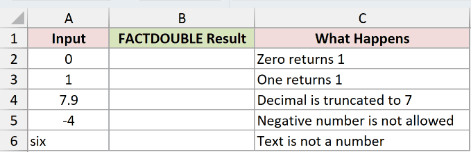
We want to see how FACTDOUBLE handles zero, one, a decimal, a negative number, and text.
Here is the formula:
=FACTDOUBLE(A2)
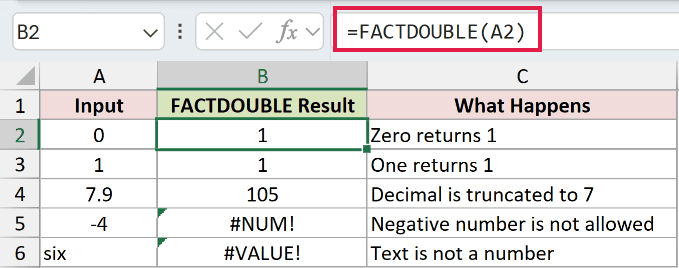
Enter the formula in B2 and fill it down to B6. The first two inputs, 0 and 1, both return 1.
The decimal 7.9 in A4 is truncated to 7. B4 therefore returns 105, the product of 7 × 5 × 3 × 1.
The negative input -4 returns #NUM! in B5. The text “six” returns #VALUE! in B6 because it is not a number.
Pro Tip: Truncation is different from rounding. FACTDOUBLE treats 7.9 as 7, so it uses the odd-number sequence rather than rounding up to the even number 8.
Tips & Common Mistakes
- Read the notation correctly. The expression n!! means double factorial, not n! multiplied by two or a factorial calculated twice.
- Check the input before hiding an error. Negative numbers return #NUM!, while nonnumeric text returns #VALUE!. A bare range can also cause #VALUE!, as Example 2 shows.
- Leave room for spilled results. Occupied output cells can cause #SPILL!. Enter the array formula only in its starting cell.
- Remember the version difference. The spill examples need Excel 2021, Excel 2024, or Microsoft 365. In older versions, calculate one row at a time and fill down.
- Use the even-number identity as a check. For a nonnegative integer k, (2k)!! equals 2^k × k!. This separates the factor of 2 from each even number.
- PRODUCT and SEQUENCE can expose the factors. For positive integer inputs, they can generate and multiply a sequence stepping down by two. FACTDOUBLE expresses the same task more directly.
- Large results have limits. Double factorials grow quickly and can exceed Excel’s numeric capacity, producing #NUM!.
Related Excel Functions / Articles:
