
Excel’s IMCOSH function returns the hyperbolic cosine of a complex number. It accepts values with real and imaginary parts, such as 4+3i.
You might use it in a transmission-line calculation where the input includes both attenuation and phase. The result stays in complex-number text form, ready for other complex functions.
Even when its answer looks like an ordinary number, IMCOSH returns text. That matters when you want to format the answer or use it in further calculations.
I’ll show you how to compare IMCOSH with COSH, check its relationship with IMCOS, and calculate a transmission line’s no-load voltage rise.
IMCOSH Function Syntax in Excel
IMCOSH takes a complex number as its argument:
=IMCOSH(inumber)
- inumber (required): The complex number to evaluate. You can supply a cell reference, a real number, or complex text using a lowercase
iorjsuffix. COMPLEX builds that text from real and imaginary coefficients.
When typing complex text directly into a formula, surround it with double quotes. When the text is already in a cell, reference that cell without quotes.
IMCOSH is available in Excel 2013 and later.
When to Use IMCOSH Function
- Calculate hyperbolic cosines when your inputs contain imaginary parts.
- Check a complex calculation against the equivalent cosine identity.
- Calculate the A parameter in a transmission-line model, then extract its magnitude for a voltage calculation.
For entirely real inputs, COSH is usually the better choice because it returns an ordinary number.
Example 1: Calculate Complex Hyperbolic Cosines
Let’s start with a column containing both lowercase suffixes and a few sign changes.
Below is the dataset. Column A contains complex numbers, and column B has the Hyperbolic Cosine header with empty cells for the results.
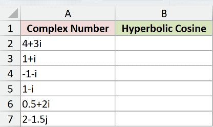
We want to calculate the hyperbolic cosine of each value in column A.
Enter this formula in B2, then copy it down to B7:
=IMCOSH(A2)
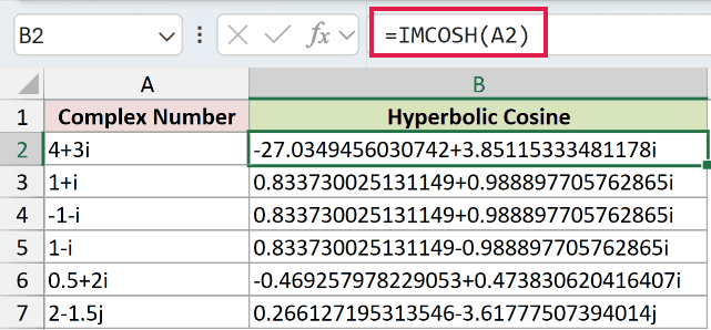
For 4+3i, the formula returns -27.0349456030742+3.85115333481178i. Excel keeps the real and imaginary parts together as text.
The inputs 1+i and -1-i both return 0.833730025131149+0.988897705762865i. Reversing both signs leaves the hyperbolic cosine unchanged.
Changing only the imaginary sign, from 1+i to 1-i, returns 0.833730025131149-0.988897705762865i. The result’s imaginary sign changes too.
The last input, 2-1.5j, returns 0.266127195313546-3.61777507394014j. IMCOSH preserves the lowercase j suffix.
Pro Tip: Bare ranges return one #VALUE!. A leading + enables spilling in Excel 2021, Excel 2024 and Microsoft 365. In Excel 2019 and earlier, use per-row formulas.
Example 2: Compare IMCOSH With COSH
For real inputs, IMCOSH returns text and COSH returns a number.
Below is the dataset. Column A contains real numbers, column B is reserved for IMCOSH results, and column C holds the COSH comparison.
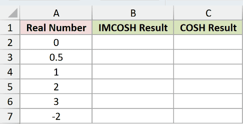
We want to compare the complex function’s text output with COSH’s numeric output.
Enter this formula in B2 and copy it down to B7:
=IMCOSH(A2)
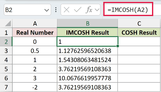
For the input 1, IMCOSH returns the text 1.54308063481524. There is no imaginary part in the answer, so Excel leaves off the suffix.
For the COSH comparison, enter this formula in C2 and copy it down to C7:
=COSH(A2)
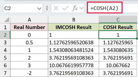
The COSH comparison displays 1.543080635 for that input. It represents the same mathematical result, but the numeric cell’s General format displays fewer digits here.
For the input 0, both columns display 1. The IMCOSH answer is still text, while the COSH comparison is a number.
Use COSH for real-number calculations. Its numeric results work with ordinary number formatting and arithmetic without extracting a component first.
For other real-number calculations, COS returns the ordinary cosine, while TANH returns the hyperbolic tangent.
Example 3: Check the Complex Cosine Identity
The hyperbolic cosine of a complex number equals the cosine of that number multiplied by the imaginary unit.
Below is the dataset. Column A contains complex inputs; columns B through E provide spaces for the identity-check helper, IMCOSH result, IMCOS comparison, and equality check.
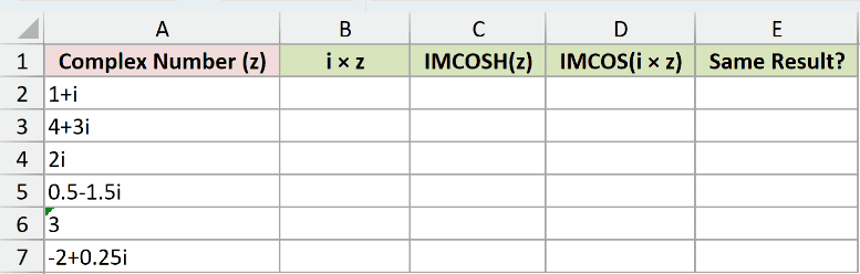
We want to check that IMCOSH agrees with the IMCOS route for each input.
For the identity-check helper, enter this in B2 and copy it down to B7:
=IMPRODUCT("i",A2)
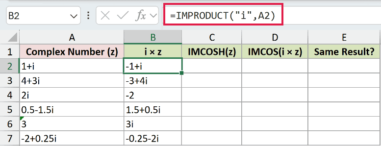
IMPRODUCT performs complex multiplication. The identity-check helper turns the first input, 1+i, into -1+i.
Calculate the direct result in C2, then copy down to C7:
=IMCOSH(A2)
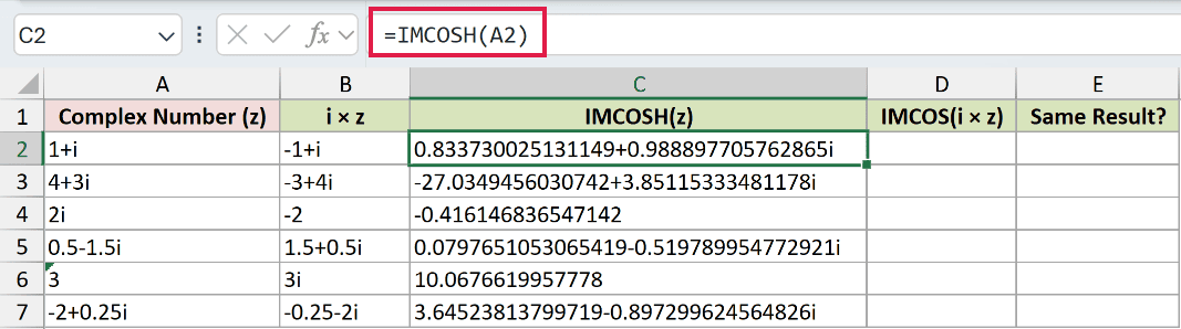
The first result is 0.833730025131149+0.988897705762865i.
For the identity comparison, enter this formula in D2 and copy it down to D7:
=IMCOS(B2)
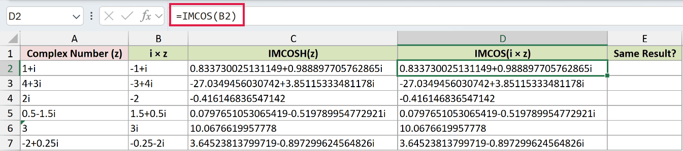
The IMCOS check also returns 0.833730025131149+0.988897705762865i in the first row.
Finally, enter the equality check in E2 and copy it down to E7:
=C2=D2
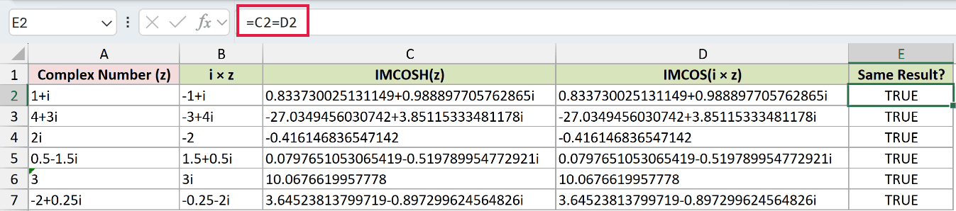
Every identity check returns TRUE for these inputs. Columns B, D and E support the check; they aren’t additional answers to calculate separately.
The pure imaginary input 2i returns -0.416146836547142 through both routes. Its hyperbolic cosine is real, although IMCOSH still stores that answer as text.
Example 4: Calculate No-Load Voltage Rise
In a long-line model, the A parameter is the hyperbolic cosine of propagation constant times length. Its magnitude determines the receiving-to-sending voltage ratio at no load.
Below is the dataset. Each transmission line has a length and propagation constant, with columns D and E reserved for the A parameter and no-load voltage rise.
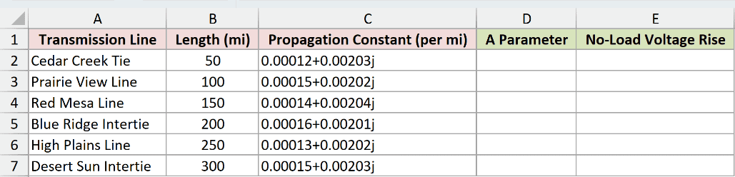
We want to calculate each line’s complex A parameter, then turn it into a usable percentage.
Enter this formula in D2 and copy it down to D7:
=IMCOSH(IMPRODUCT(B2,C2))
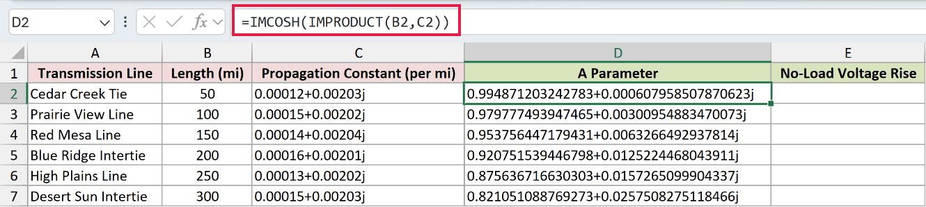
IMPRODUCT multiplies the length by its complex propagation constant. IMCOSH then calculates the hyperbolic cosine of that product.
Cedar Creek Tie returns 0.994871203242783+0.000607958507870623j in D2.
Next, enter this formula in E2 and copy it down to E7:
=1/IMABS(D2)-1
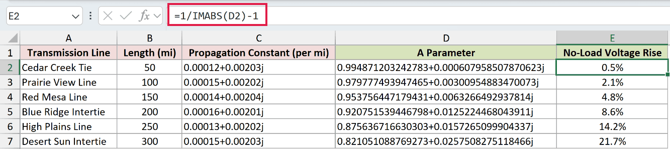
IMABS extracts the A parameter’s magnitude as a number. Taking its reciprocal and subtracting 1 converts the voltage ratio into a rise.
Format column E as a percentage. Cedar Creek Tie shows 0.5%, Prairie View Line shows 2.1%, and Desert Sun Intertie shows 21.7%.
Keep the units consistent: the lengths here are in miles, so the propagation constants are per mile.
Example 5: Diagnose IMCOSH Errors
An invalid complex string and an excessively large real part can produce the same error for different reasons.
Below is the dataset. Column A names each test case, column B contains its input, and column C is reserved for results, including deliberate errors.
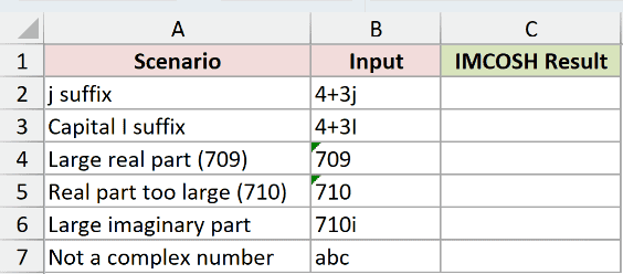
We want to distinguish valid inputs from suffix errors, overflow, and ordinary text.
Enter this formula in C2 and copy it down to C7:
=IMCOSH(B2)
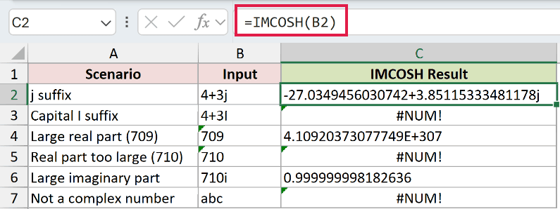
Read each row separately:
- Lowercase j:
4+3jreturns-27.0349456030742+3.85115333481178j. The suffix is accepted and preserved. - Capital I:
4+3Ideliberately returns#NUM!inC3. Change the suffix to lowercasei. - Large real part:
709returns4.10920373077749E+307. Scientific notation here represents a valid, very large result. - Real part too large:
710deliberately returns#NUM!inC5because the calculation overflows. - Large imaginary part:
710ireturns0.999999998182636. A large imaginary part does not cause the same overflow as a large real part. - Ordinary text:
abcdeliberately returns#NUM!inC7because it isn’t a complex number. Correct the source input.
The error cells are intentional demonstrations. Their result styling doesn’t make them valid answers.
Tips & Common Mistakes
- Keep complex results as text until you need a component. IMREAL extracts the real part, IMAGINARY extracts the imaginary coefficient, and IMABS returns the magnitude as a number.
- Number formats won’t shorten complex text. Widen the column to read the result; changing the decimal format doesn’t round an IMCOSH string.
- Use complex arithmetic functions for complex text. IMPRODUCT handles multiplication, and IMSUM handles addition. Ordinary SUM isn’t the right way to total these results.
- Check the input before hiding an error. A capital suffix, invalid text, and overflow need different corrections, even when each produces
#NUM!.
Other Excel articles you may also like:
