
The IMSIN function in Excel returns the sine of a complex number as text, keeping its real and imaginary parts together in the result.
That makes it useful when your input contains an imaginary component. Unlike ordinary sine, a complex sine can have a magnitude greater than 1.
Even when the answer looks like an ordinary number, IMSIN still returns text. For real angles that you’ll use in everyday calculations, SIN is usually the better choice.
I’ll show you how to calculate complex sines, compare IMSIN with SIN, and check what happens with purely imaginary inputs.
IMSIN Function Syntax in Excel
IMSIN takes a complex number as its required argument:
=IMSIN(inumber)
- inumber (required): The complex number whose sine you want. Supply complex text using lowercase
iorj, a cell reference, or a value built with COMPLEX.
A complex number has a real part and an imaginary part. In 4+3i, those parts are 4 and 3.
IMSIN also accepts real numbers and purely imaginary values. For real angles entered in degrees, convert them to radians first with RADIANS.
When to Use IMSIN Function
- Calculate the sine of complex numbers stored in a worksheet column.
- Work with purely imaginary inputs and examine how their sines grow.
- Calculate a complex sine from separate real and imaginary input columns.
- Check complex sine calculations against their real and imaginary components.
Example 1: Calculate Sines of Complex Numbers
Let’s start with a column that shows how changing the input changes its sine.
Below is the dataset. Column A describes each case, column B holds complex inputs, and columns C and D have space for sines and their magnitudes.
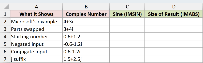
We want to calculate each complex sine, then measure the size of the result.
Enter this formula in C2 and copy it down to C7:
=IMSIN(B2)
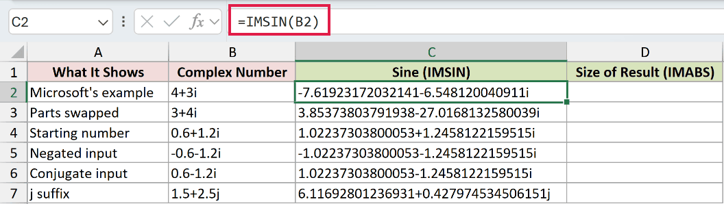
For 4+3i, the result is -7.61923172032141-6.548120040911i. Swapping the input parts to 3+4i returns 3.85373803791938-27.0168132580039i.
The starting input 0.6+1.2i returns 1.02237303800053+1.2458122159515i. Negating the entire input returns -1.02237303800053-1.2458122159515i, reversing both signs.
Changing only the imaginary sign creates the conjugate input, 0.6-1.2i. Its sine is 1.02237303800053-1.2458122159515i, with only the imaginary sign reversed.
The last row also shows that Excel keeps the suffix: 1.5+2.5j returns 6.11692801236931+0.427974534506151j.
To measure each sine’s magnitude, enter this formula in D2 and copy it down to D7:
=IMABS(C2)
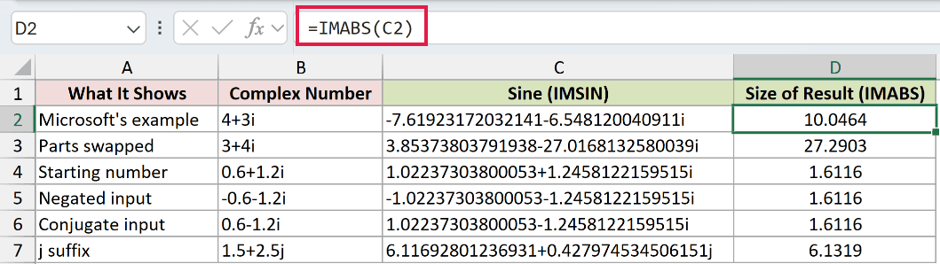
IMABS returns a number representing the complex result’s size. The first magnitudes are 10.0464 and 27.2903, so complex sine isn’t limited to ordinary sine’s bounds.
The starting, negated, and conjugate inputs all produce the same magnitude, 1.6116.
These formulas are entered per row and copied down. Passing a bare range to IMSIN returns a single #VALUE! error instead of filling the output column.
Pro Tip: In Excel 2021, Excel 2024 and Microsoft 365, =IMSIN(+B2:B7) or =IMSIN(B2:B7&"") coerces the range into an array so the results spill.
In Excel 2019 and earlier, copy the per-row formula down instead.
Example 2: Compare IMSIN With SIN
For real angles, the main difference is the type of result you receive.
Below is the dataset. Column A contains angles in degrees, column B will hold IMSIN results, and column C is the real-number SIN comparison.
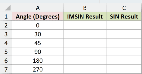
We want to compare complex-text sine results with ordinary numeric sine results for the same angles.
Enter this formula in B2 and copy it down to B7:
=IMSIN(RADIANS(A2))
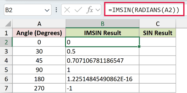
RADIANS converts each degree input before IMSIN calculates its sine. The 30-degree row returns 0.5, and the 45-degree row returns 0.707106781186547.
Both are text, even though neither contains an imaginary suffix. The 90-degree result, 1, is text too.
For the real-number comparison, enter this formula in C2 and copy it down to C7:
=SIN(RADIANS(A2))
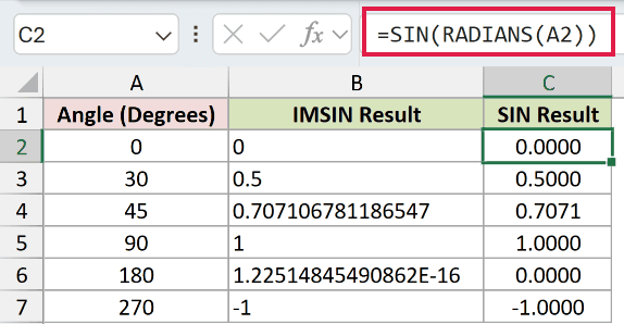
The SIN comparison displays 0.5000 for 30 degrees and 0.7071 for 45 degrees. These are numbers, so the column’s number format controls their displayed decimals.
Changing the number format doesn’t shorten IMSIN’s text. Use SIN when your inputs are real angles and you need numeric results for further calculations.
At 180 degrees, IMSIN returns 1.22514845490862E-16. That’s a tiny floating-point rounding residue, effectively zero, rather than an error.
The SIN comparison displays 0.0000 on that row because its number format hides the residue. A displayed zero doesn’t mean the stored result is exactly zero.
At 270 degrees, IMSIN returns the text -1, while the SIN comparison displays the number as -1.0000.
Example 3: Work With Purely Imaginary Inputs
A purely imaginary input produces a purely imaginary sine, and its size can grow quickly.
Below is the dataset. Column A holds purely imaginary inputs, column B is reserved for IMSIN, and column C holds a SINH identity check.
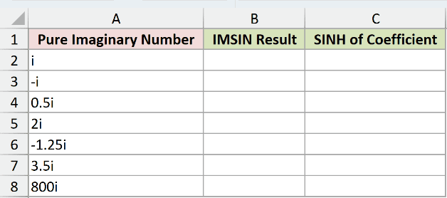
We want to calculate each sine and check its imaginary coefficient against the hyperbolic sine of the input coefficient.
Enter this formula in B2 and copy it down to B8:
=IMSIN(A2)
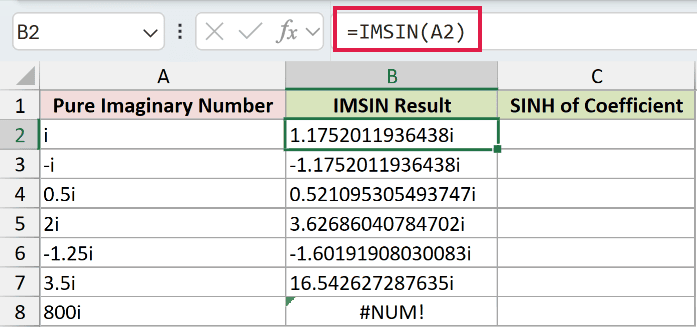
The input i returns 1.1752011936438i, while -i returns -1.1752011936438i. The sign changes with the input.
For 2i, the result is 3.62686040784702i. By 3.5i, it has grown to 16.542627287635i.
For a purely imaginary input yi, the sine is i multiplied by the hyperbolic sine of y. SINH calculates that real coefficient.
Enter the identity-check formula in C2 and copy it down to C8:
=SINH(IMAGINARY(A2))
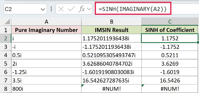
IMAGINARY extracts the input’s imaginary coefficient, then SINH calculates its hyperbolic sine. Column C provides a numeric check of the sine’s imaginary coefficient.
The check displays 1.1752 beside the input i and 16.5426 beside 3.5i. Those numbers match the imaginary coefficients, rounded for display.
The final input, 800i, deliberately produces #NUM! in B8. Its imaginary part makes the sine too large for Excel to represent.
The identity check in C8 also deliberately returns #NUM!, because SINH overflows on that coefficient. Neither error indicates incorrectly written complex text.
Pro Tip: This overflow comes from the large imaginary part. IMSIN accepts the real input 800 without an overflow error.
Example 4: Check the Parts Behind IMSIN
Now let’s see how the real and imaginary input parts contribute to the answer.
Below is the dataset. Columns A and B contain separate input parts, column C will hold IMSIN results, and columns D and E are identity checks.
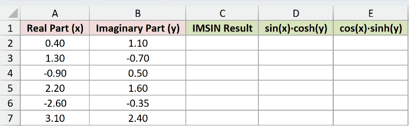
We want to build each complex input, calculate its sine, and independently check the real and imaginary parts of that result.
Enter this formula in C2 and copy it down to C7:
=IMSIN(COMPLEX(A2,B2))
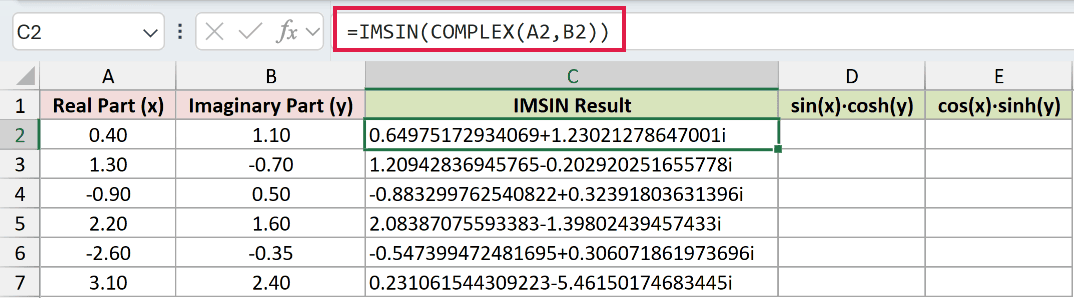
COMPLEX joins the real part in A2 and imaginary part in B2 into complex text. IMSIN then calculates the sine.
The first row, with inputs 0.40 and 1.10, returns 0.64975172934069+1.23021278647001i.
The real part of a complex sine is sin(x) multiplied by cosh(y). Enter this identity check in D2 and copy it down to D7:
=SIN(A2)*COSH(B2)
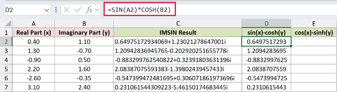
The real-part check displays 0.6497517293 in D2. It matches the real part of C2 to the displayed precision.
The imaginary coefficient is cos(x) multiplied by sinh(y). Enter this identity check in E2 and copy it down to E7:
=COS(A2)*SINH(B2)
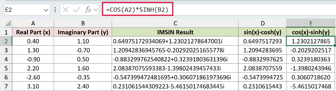
The imaginary-part check displays 1.2302127865 in E2, matching the imaginary coefficient in C2 to the displayed precision.
Columns D and E verify the components of the answer in column C. IMSIN already performs this calculation, so you don’t need these checks in ordinary use.
Tips & Common Mistakes
- Use lowercase suffixes. IMSIN accepts
iandj, but a capitalIreturns#NUM!. Malformed complex text also returns#NUM!. - Check logical inputs separately. TRUE returns
#VALUE!. A blank input silently returns the text0, so missing data can look like a valid sine. - Don’t blame spaces automatically. Excel accepts spaces within complex text. Check the suffix and arrangement of the real and imaginary parts first.
- Extract numbers before ordinary math. IMREAL and IMAGINARY return numeric components; IMABS returns a numeric magnitude. IMSIN’s complex text cannot be summed directly or rounded by changing its number format.
- Keep degrees and radians straight. Convert real degree inputs with RADIANS, as in Example 2. Don’t apply RADIANS to a complete complex-text value.
- Keep range behavior in mind. The examples use per-row formulas because bare ranges fail. MAP with LAMBDA is another array route in Microsoft 365 and Excel 2024.
Other Excel articles you may also like:
