
The IMREAL function in Excel returns the real part of a complex number as a number you can use in ordinary calculations.
In complex notation, the real part is the component without the i or j suffix. For a wiring impedance, that component represents resistance.
Because IMREAL returns a number, you can add its results with SUM or compare them against a limit without converting text first.
I’ll show you how to extract real parts, total movement from complex values, and filter wiring runs by resistance, including the input mistakes to watch for.
IMREAL Function Syntax in Excel
IMREAL takes a complex value and extracts its real component:
=IMREAL(inumber)
- inumber (required): The complex value to read, usually text in
x+yiorx+yjform. You can supply a cell reference, quoted text, or another function’s result.
Use lowercase i or j for the imaginary suffix. When entering complex text directly inside a formula, put it in double quotes. Cell references don’t need quotes.
When to Use IMREAL Function
- Extract signed real components from a list of complex values.
- Add horizontal movements stored as complex route coordinates.
- Classify control-loop responses using the sign of a pole’s real part.
- Filter impedance readings by their resistance component.
Example 1: Extract the Real Part
Let’s start with a column containing different complex-number forms.
Below is the dataset. Column A contains complex values, and the Real Part header in column B marks where the extracted numbers will appear.
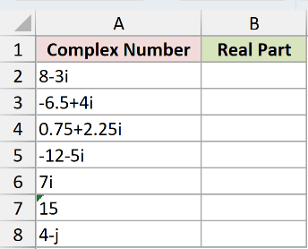
We want to extract each value’s real component while keeping its sign and decimal places.
Enter this formula in B2, then copy it down through B8:
=IMREAL(A2)
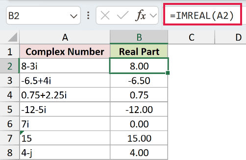
The first input, 8-3i, returns 8.00. The negative input -6.5+4i returns -6.50, and 0.75+2.25i returns 0.75.
The remaining rows show the other useful cases:
-12-5ireturns -12.00. The imaginary component doesn’t change the real component’s sign.7ireturns 0.00 because it has no real component.- The text value
15returns 15.00. A suffix isn’t required for a purely real value. 4-jreturns 4.00, so lowercasejworks too.
These are numeric results. The decimal formatting in column B controls their appearance, so you can format them like other worksheet numbers.
Example 2: Sum Real Parts Across a Range
A robot’s route can store horizontal and vertical movement together as complex text.
Below is the dataset. Columns A:B list robot legs and moves; column C will hold east-west movement, and E2 will hold the net movement.
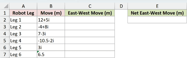
We want each leg’s east-west movement and the net movement across the route.
Here, a positive real part means east and a negative real part means west. The imaginary component represents north-south movement.
Enter this formula in C2:
=IMREAL(+B2:B7)
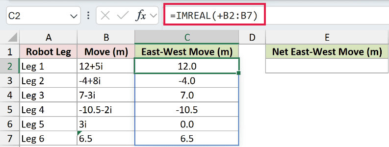
The results spill into C2:C7: 12.0, -4.0, 7.0, -10.5, 0.0, and 6.5.
The leading + makes Excel pass the range’s values as an array. A bare range passed directly to IMREAL returns a single #VALUE! error instead.
This spill works in Excel 2021, Excel 2024, and Microsoft 365. In Excel 2019 and earlier, extract each row separately and copy down.
Pro Tip: In Microsoft 365 and Excel 2024 only, you can also use =MAP(B2:B7,LAMBDA(z,IMREAL(z))). MAP passes each value to IMREAL separately and spills the results, so the leading + is unnecessary.
Now enter the total formula in E2:
=SUM(IMREAL(+B2:B7))
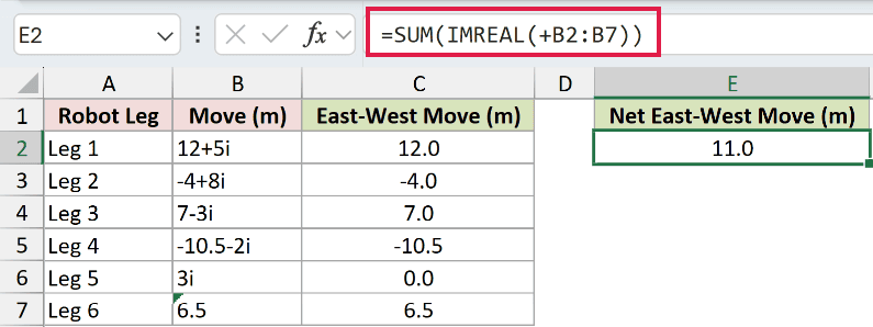
E2 returns 11.0 meters. Because the result is positive, the robot finishes that far east of its starting position.
IMREAL extracts the real components inside the formula, and SUM adds them. This returns a single-cell total without needing the helper column in C.
The total measures the change in east-west position. Westward legs reduce it; distance traveled counts the length of every leg.
Example 3: Classify Control-Loop Responses
The sign of a pole’s real part can also drive a decision.
Below is the dataset. Columns A:B list control loops and dominant poles, with Real Part and Response headers in columns C:D for the calculations.
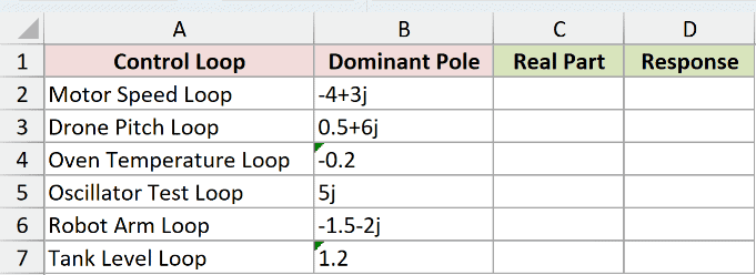
We want to label each listed continuous-time response using its dominant pole’s real part.
First, enter this formula in C2 and copy it down through C7:
=IMREAL(B2)
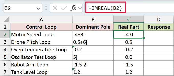
Motor Speed Loop returns -4.0, Drone Pitch Loop returns 0.5, and Oscillator Test Loop returns 0.0.
For the cases shown, negative real parts indicate decaying, stable responses. Positive real parts indicate growing, unstable responses; the pure imaginary pole represents marginal stability.
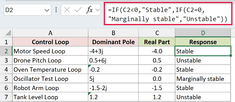
Enter this classification formula in D2 and copy it down through D7:
=IF(C2<0,"Stable",IF(C2=0,"Marginally stable","Unstable"))
How this formula works:
- The first IF checks whether C2 is negative and returns Stable when it is.
- Otherwise, the second IF checks for zero and returns Marginally stable.
- A positive value reaches the final branch and returns Unstable.
Motor Speed Loop, Oven Temperature Loop, and Robot Arm Loop return Stable. Drone Pitch Loop and Tank Level Loop return Unstable.
Oscillator Test Loop returns Marginally stable because its 5j pole has a real part of 0.0.
Both columns use copied-down formulas. Each Response cell checks the numeric Real Part cell on its own row.
Example 4: Filter Wiring Runs by Resistance
For an impedance reading, IMREAL extracts the resistance component.
Below is the dataset. Columns A:B contain wiring runs and impedances, D2 holds the resistance limit, and column F is reserved for runs over that limit.
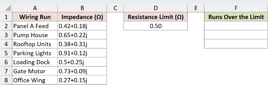
We want the wiring-run names whose resistance exceeds the limit entered in D2.
Enter this formula in F2:
=FILTER(A2:A8,IMREAL(+B2:B8)>D2)
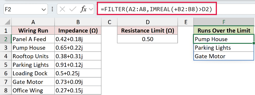
FILTER is available in Excel 2021 and later.
The names Pump House, Parking Lights, and Gate Motor spill into F2:F4.
How this formula works:
- The leading
+passes the impedance values to IMREAL as an array. - IMREAL extracts the resistance component from each value.
- The
>comparison checks each resistance against D2. - FILTER returns the corresponding names from A2:A8 when that comparison is true.
The limit in D2 displays 0.50 ohms. Loading Dock is exactly 0.5 ohms, so it isn’t over the limit and doesn’t appear.
D2 is a typed input. Change it to apply a different resistance limit without editing the formula.
Example 5: Check Accepted Inputs and Errors
Some unusual-looking inputs work, while others produce deliberate errors in this example.
Below is the dataset. Column A labels each input type, column B contains the test inputs, and column C is set up for the real-part results.
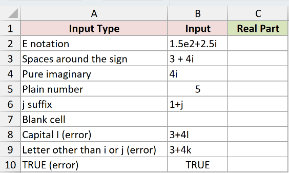
We want to see which inputs IMREAL accepts and distinguish invalid text from an invalid logical value.
Enter this formula in C2 and copy it down through C10:
=IMREAL(B2)
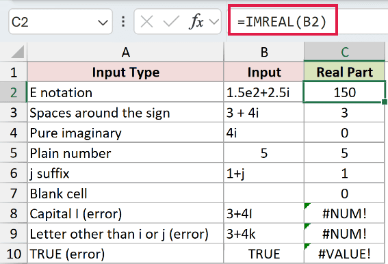
Each row demonstrates a different input case:
- E notation, row 2:
1.5e2+2.5ireturns 150. IMREAL reads scientific notation in the real component. - Spaces, row 3:
3 + 4ireturns 3. The spaces around the sign don’t make this input invalid. - Pure imaginary, row 4:
4ireturns 0 because there’s no real component. - Plain number, row 5: The numeric input
5returns 5. - Lowercase j, row 6:
1+jreturns 1, confirming that this suffix is accepted. - Blank cell, row 7: The empty B7 returns 0. This silently turns a missing input into a zero that could be mistaken for a measured reading.
- Capital I, row 8:
3+4Ideliberately returns #NUM! in C8. Replace the uppercase suffix with lowercasei. - Wrong suffix, row 9:
3+4kdeliberately returns #NUM! in C9. Use lowercaseiorjinstead ofk. - Logical input, row 10:
TRUEdeliberately returns #VALUE! in C10 because it isn’t a supported numeric or complex-text input.
Pro Tip: Check missing inputs before treating the output as a reading. The blank B7 and the pure imaginary input both return 0, but they mean different things.
Tips & Common Mistakes
- Keep the range conversion. Example 2’s leading
+matters. Removing it passes a bare range, which IMREAL rejects with#VALUE!. - Choose the component you need. IMREAL extracts the real part, IMAGINARY extracts the imaginary coefficient, and IMABS returns the magnitude.
- Build a complex value from its parts. COMPLEX builds complex text from separate real and imaginary components. IMREAL extracts a number from that text.
- Read other complex-function results directly. IMREAL can extract the real component from text returned by functions such as IMSUM or IMLN.
- Diagnose the input before hiding an error. Unsupported complex text and logical values cause different errors, as the final example shows.
Related Excel Functions / Articles:
