
The SECH function in Excel returns the hyperbolic secant of a number.
Its symmetric curve peaks at input 0, where the result is 1, and falls toward zero in either direction.
That shape makes SECH useful for modeling a pulse that rises to a central peak and then fades. Positive and negative inputs of the same size return matching results.
I’ll show you how to calculate SECH over a list, build a pulse profile, and compare its behavior with equivalent calculations at large inputs.
SECH Function Syntax in Excel
SECH takes a single required argument:
=SECH(number)
- number (required): The real number you want to evaluate. You can supply a number, a cell reference, or a range.
The input isn’t an angle, so don’t convert it from degrees to radians. SECH is available in Excel 2013 and later.
When to Use SECH Function
- Calculate hyperbolic secant values for a mathematical model.
- Build a symmetric pulse profile using a peak value and a width parameter.
- Evaluate very large inputs without the overflow errors that equivalent calculations can produce.
- Calculate a curve’s slope when your model specifies the square of the hyperbolic secant.
Example 1: Calculate SECH for a List
Let’s start with positive and negative inputs to see the symmetry directly.
Below is the dataset. Column A contains the numbers, column B will hold SECH results, and column C provides a comparison showing recovered input magnitudes.
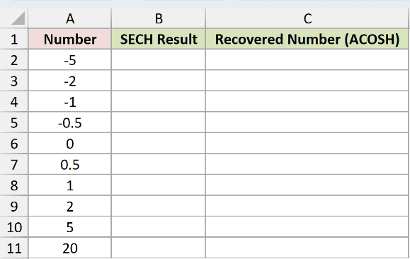
We want to calculate the hyperbolic secant of every number in column A.
Enter this formula in B2:
=SECH(A2:A11)
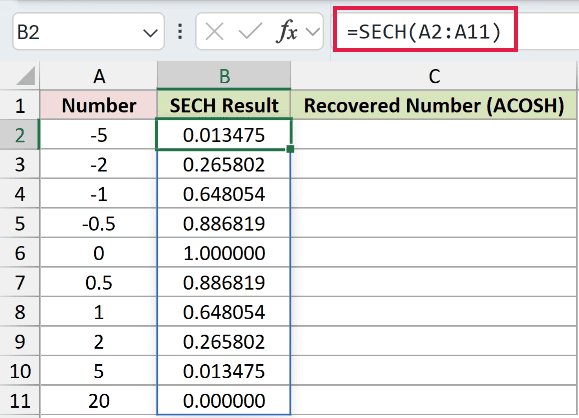
The results spill into B2:B11 in Excel 2021, Excel 2024, and Microsoft 365. In Excel 2019 and earlier, use a single-cell reference and copy down.
Both -2 and 2 return 0.265802. At the center, the input 0 returns 1.000000, the highest result in the column.
As the input moves farther from zero, the result becomes smaller. The inputs -5 and 5 both return 0.013475.
Now let’s check whether we can recover the original inputs. ACOSH returns an inverse hyperbolic cosine; applying it to the reciprocal of a SECH result recovers the input’s magnitude.
Enter this comparison formula in C2:
=ACOSH(1/B2:B11)
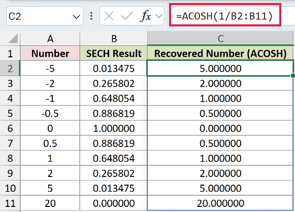
The comparison spills into C2:C11. The original -5 becomes 5.000000, and -2 becomes 2.000000. Positive inputs keep their magnitude, while zero returns 0.000000.
SECH loses the input’s sign because opposite inputs share the same result. Excel has no dedicated inverse hyperbolic secant function.
Pro Tip: B11 displays 0.000000, but its stored result is still positive. That’s why the comparison in C11 can recover 20.000000. Use scientific formatting when small values look like zero.
Example 2: Model a Bell-Shaped Light Pulse
Squaring SECH lets us build a pulse profile around a central peak.
Below is the dataset. Column A lists times in picoseconds, column B will hold power, and the card in columns D and E contains peak and width inputs.
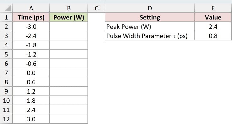
We want to calculate the pulse’s power at each listed time.
The card contains typed inputs: 2.4 watts in E2 and a width parameter of 0.8 picoseconds in E3.
Enter this formula in B2:
=$E$2*SECH(A2:A12/$E$3)^2
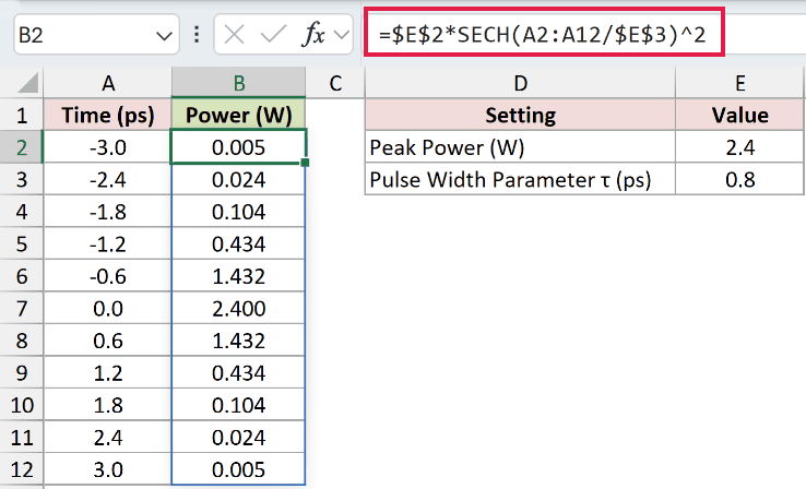
The power values spill into B2:B12.
How this formula works:
- Dividing the times by
$E$3expresses each time relative to the width parameter. Both use picoseconds, so the input to SECH has no units. - SECH calculates the symmetric profile, and the exponent squares each result.
- Multiplying by
$E$2scales the profile to the specified peak power in watts.
At time 0.0, the calculated power is 2.400 watts. At -0.6 and 0.6 picoseconds, both results are 1.432 watts.
The outer times, -3.0 and 3.0, both return 0.005 watts. The matching pairs show the pulse fading equally on either side of its peak.
Changing the peak input scales the power values. Changing the width parameter makes the pulse broader or narrower while keeping its center in place.
Example 3: Compare SECH With Equivalent Formulas
Let’s compare SECH with reciprocal and exponential calculations, including inputs past 709.
Below is the dataset. Column A contains test numbers, column B will hold SECH results, and columns C and D are reserved for equivalent-formula comparisons.
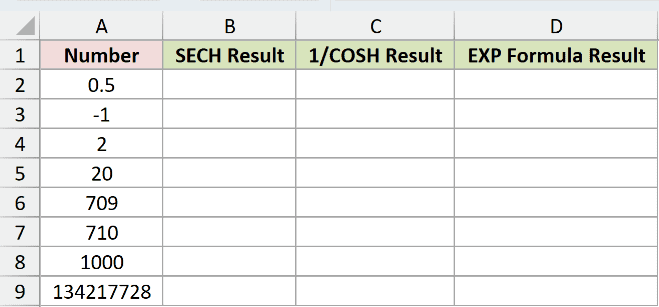
We want to compare SECH with manual calculations, including inputs large enough to expose overflow.
Enter the SECH formula in B2:
=SECH(A2:A9)
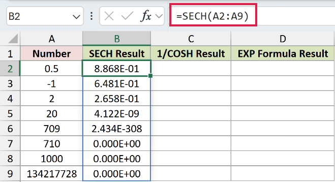
The result for 20 is 4.122E-09, and 709 returns 2.434E-308. Scientific formatting keeps these very small values visible.
For the tested inputs 710, 1000, and 134217728, SECH returns 0.000E+00 without an error.
COSH calculates the hyperbolic cosine. Its reciprocal is mathematically the hyperbolic secant, so we can use it to check SECH’s results.
Enter this comparison formula in C2:
=1/COSH(A2:A9)
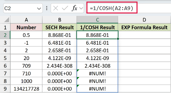
The comparison matches SECH through 709, including 2.434E-308. But the deliberate error demonstrations in C7:C9 return #NUM! because the intermediate hyperbolic cosine overflows.
EXP raises the mathematical constant e to a power. Combining positive and negative exponential terms provides another expression for the hyperbolic secant.
Enter this second comparison formula in D2:
=2/(EXP(A2:A9)+EXP(-A2:A9))
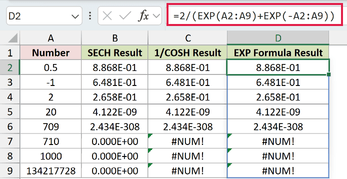
This comparison also matches SECH through 709. The deliberate error cells in D7:D9 show #NUM! because the exponential calculation overflows.
The #NUM! cells show where intermediate values exceed Excel’s numerical limits. SECH returns zero for those same inputs.
Example 4: Calculate a Curve’s Slope
SECH squared also describes how quickly a hyperbolic tangent curve changes.
TANH returns the hyperbolic tangent, which forms an S-shaped curve. Its slope at each input equals the square of SECH at that input.
Below is the dataset. Column A contains inputs, columns B through D provide curve and slope scaffolding, and the card in F:G holds a step size.
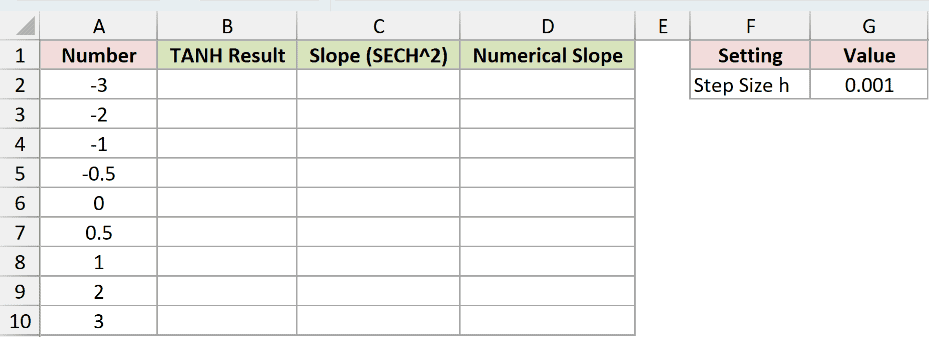
We want to calculate the slope with SECH and compare it with an estimate from nearby curve values.
First, enter the supporting curve formula in B2:
=TANH(A2:A10)
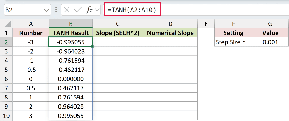
The curve values spill into B2:B10. At -3, the curve returns -0.995055; at 3, it returns 0.995055.
Now enter the SECH slope formula in C2:
=SECH(A2:A10)^2
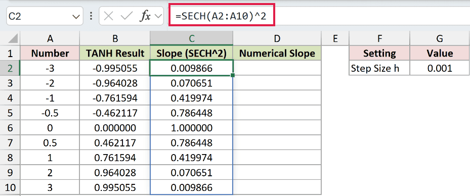
The slopes spill into C2:C10. At input 0, the slope is 1.000000. At -3 and 3, it is only 0.009866.
So the curve changes fastest at its center and flattens toward either end. The slope stays positive even where the curve values themselves are negative.
For a numerical comparison, G2 holds the typed step size 0.001. We’ll sample the curve just above and below each input.
Enter the comparison formula in D2:
=(TANH(A2:A10+$G$2)-TANH(A2:A10-$G$2))/(2*$G$2)
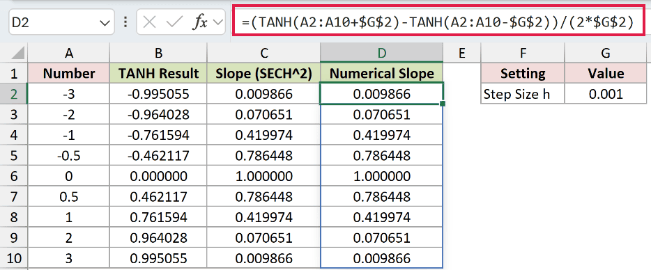
The numerator subtracts the nearby curve values. The denominator is the distance between those sample points, so dividing estimates the slope.
The comparison in column D matches column C at the displayed precision. For example, both show 0.419974 at input 1 and 0.070651 at input 2.
Column D estimates the slope using a small step and matches column C to the displayed six decimals. The SECH expression calculates the derivative directly.
Tips & Common Mistakes
- Don’t convert angles. SECH takes a plain number. In a model like the pulse example, divide quantities with matching units before passing the result to SECH.
- Check empty inputs. A reference to an empty cell is treated as zero, so SECH returns 1. Missing data can therefore look like a valid peak.
- Watch text and logical values. Numeric text is converted to a number, and TRUE is treated as 1. Text such as
abcreturns#VALUE!. - Keep spill destinations clear. Occupied output cells can cause
#SPILL!. Enter each range formula only in its starting cell and let Excel populate the remaining cells. - Check unexpected single results. An
@operator can reduce a range calculation to a single value instead of allowing the results to spill. - Distinguish tiny values from zeros. Scientific formatting reveals small stored values hidden by decimal formatting. It won’t turn an actual zero into a nonzero result.
Related Excel Functions / Articles:
