
An annuity is a series of equal payments made at regular intervals, like a monthly payout from a retirement annuity or a fixed deposit into a savings plan.
Excel handles annuities with a small group of financial functions. Each solves for one unknown: the payment, the value today, the value later, the number of payments, or the rate.
Two things trip people up. The rate and the number of periods have to be on the same schedule.
And payments at the start of a month give a different answer than payments at the end.
In this article, I’ll show you how to work out the monthly payout from a lump sum, the lump sum behind a monthly income, and what regular savings grow to.
I’ll also cover annuity due, how long the money lasts, and the math formula behind it all.
Method #1: Using the PMT Function
The most common annuity question is “how much will this pay me each month?” The PMT function answers it when you know the lump sum, the rate, and the term.
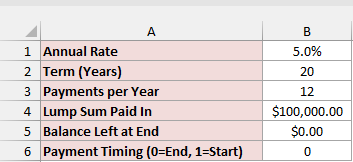
Below I have the inputs on the Payment (PMT) sheet. You pay $100,000 into an annuity that earns 5% a year and pays out monthly for 20 years.
B5 is the balance left at the end (zero, so the money is fully paid out), and B6 is the payment timing (0 means the end of each month).
Enter this formula in B7:
=PMT(B1/B3,B2*B3,-B4,B5,B6)
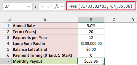
The result is $659.96 a month. So a $100,000 annuity at 5% pays about $660 a month for 20 years.
How does this formula work?
B1/B3 turns the 5% annual rate into a monthly rate, and B2*B3 turns 20 years into 240 monthly payments.
-B4 is the $100,000 lump sum. It has a minus sign because it’s money you hand over, which makes the payout you get back a positive number.
Note: Excel’s financial functions use signs to show which way money moves. Money you pay out is negative and money you receive is positive. If you enter the lump sum as a positive number, PMT returns -$659.96.
Method #2: Using the PV Function
Here’s the question the other way around. If you want a fixed monthly income, how big a lump sum do you need today? That’s what the PV function returns.
Below I have the inputs on the Present Value (PV) sheet. The goal is a $2,000 monthly payout for 20 years at 5% a year.
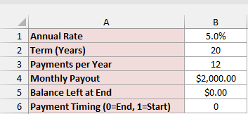
Enter this formula in B7:
=-PV(B1/B3,B2*B3,B4,B5,B6)
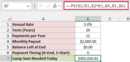
Excel returns $303,050.63. That’s the lump sum that funds $2,000 a month for 20 years at a steady 5%.
How does this formula work?
The rate and the number of periods work the same way as in PMT. B4 is the $2,000 you receive each month, so it stays positive.
PV then returns a negative number because the lump sum is money you’d pay. The minus sign before PV flips it so the answer reads as a positive amount.
Method #3: Using the FV Function
If you’re putting money in rather than taking it out, you probably want to know what it grows to. The FV function returns the balance at the end.
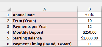
Below I have the inputs on the Future Value (FV) sheet. You start with $1,000 and add $250 at the end of every month for 10 years at 5%.
Enter this formula in B7:
=FV(B1/B3,B2*B3,-B4,-B5,B6)
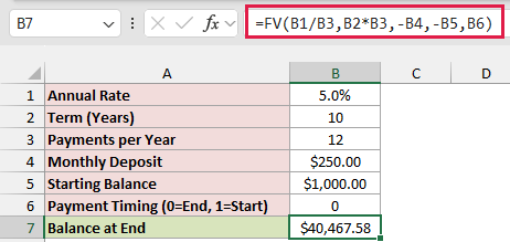
The projected balance is $40,467.58 after 10 years.
How does this formula work?
-B4 is the $250 monthly deposit and -B5 is the $1,000 starting balance. Both are money you put in, so both get a minus sign.
That makes the balance you get back at the end a positive number. If you have no starting balance, enter 0 in B5.
Method #4: Using the Type Argument (Annuity Due)
So far, every payment has happened at the end of the month. That’s an ordinary annuity. When payments happen at the start of each period, it’s an annuity due.
Rent, insurance premiums, and deposits you make on the 1st of the month are all examples of an annuity due.
PMT, PV, and FV handle this with their last argument, called type. A 0 (or leaving it out) means the end of the period, and 1 means the start.
Below I have the three examples from Methods #1 to #3 on the Annuity Due sheet, one per row, so you can compare both timings side by side.

Column F uses 0 as the last argument and column G uses 1. Here is the formula in G2 for the monthly payout:
=PMT(B2/12,C2*12,-D2,0,1)

The PV and FV rows work the same way. G3 uses =-PV(B3/12,C312,E3,0,1) and G4 uses =FV(B4/12,C412,-E4,-D4,1).
Here’s what changes when payments move to the start of the month:
- Payout: drops from $659.96 to $657.22, because the first payment goes out right away and has no time to earn interest.
- Lump sum needed: rises from $303,050.63 to $304,313.34, because each payment arrives a month sooner.
- Savings balance: rises from $40,467.58 to $40,629.33, because each deposit earns one extra month of interest.
A quick way to check an annuity due is to multiply the ordinary result by 1 plus the monthly rate. $303,050.63 times 1.0041667 gives $304,313.34.
Note: Every sheet in the example file has a Payment Timing cell (B6). Change it from 0 to 1 to turn that example into an annuity due.
Method #5: Using the NPER Function
Sometimes you know the payout you want and need to know how long the money lasts. The NPER function returns the number of payments.
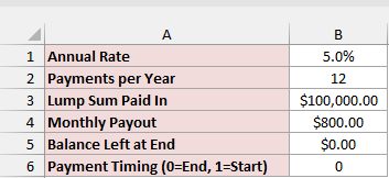
Below I have the inputs on the Number of Payments (NPER) sheet. You pay $100,000 into an annuity at 5% a year and want to take $800 a month.
Enter this formula in B7:
=NPER(B1/B2,B4,-B3,B5,B6)
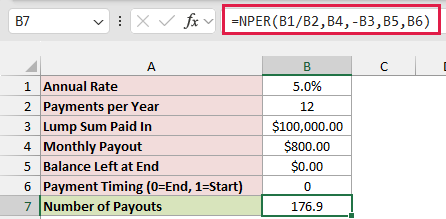
The result is 176.9 payouts. Divide it by 12 and the money lasts about 14.7 years.
How does this formula work?
B1/B2 is the monthly rate. B4 is the $800 you receive, so it’s positive, and -B3 is the $100,000 you pay in, so it’s negative.
NPER finds how many $800 payouts it takes to use up the $100,000, with interest added along the way.
Method #6: Using the RATE Function
Annuity quotes usually tell you the payout, not the return. The RATE function works backward from the payout to the interest rate.
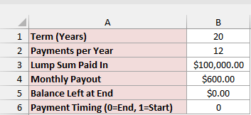
Below I have the inputs on the Interest Rate (RATE) sheet. An insurer offers $600 a month for 20 years in exchange for a $100,000 premium.
Enter this formula in B7:
=RATE(B1*B2,B4,-B3,B5,B6)*B2
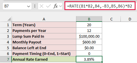
The quote works out to an annual rate of 3.89%.
How does this formula work?
B1*B2 is 240 monthly payments. B4 is the $600 payout you receive and -B3 is the premium you pay.
RATE returns the rate per period, which is monthly here. Multiplying by B2 (12) turns it into an annual rate you can compare with other quotes.
Method #7: Using the Annuity Math Formula
You don’t need a function to calculate an annuity. The present value of an annuity has a standard math formula, and Excel can work it out directly.
It’s also a handy way to see what PV is doing behind the scenes, or to check a function result.
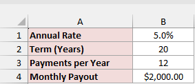
Below I have the same $2,000 monthly payout from Method #2 on the Math Formula sheet: 5% a year for 20 years.
Enter this formula in B5:
=B4*(1-(1+B1/B3)^-(B2*B3))/(B1/B3)
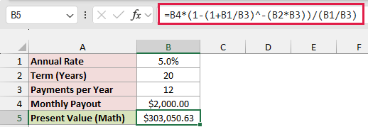
The result is $303,050.63, the same as Method #2.
How does this formula work?
This is the present value of an annuity formula: payment x (1 – (1 + r)^-n) / r.
Here r is the monthly rate (B1/B3) and n is the number of payments (B2*B3).
(1 + r)^-n discounts the last payment back to today. The rest of the formula adds up the discounted value of all 240 payments in one step.
To confirm it, I put the PV function in B6:
=-PV(B1/B3,B2*B3,B4)
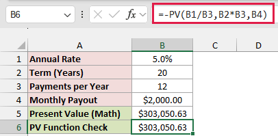
Both cells return $303,050.63.
The same idea works for the other two values. The payout is lump sum x r / (1 – (1 + r)^-n).
And the future value of regular deposits is payment x ((1 + r)^n – 1) / r.
Converting the Rate When Compounding and Payments Differ
Every example so far divides the annual rate by 12. That’s only right when the rate compounds monthly, the same as the payments.
Some annuities and savings accounts quote a rate that compounds once a year (often shown as APY) and still pay monthly. Dividing by 12 then overstates the monthly rate.
Below I have the inputs on the Rate Conversion sheet: a 5% rate compounded once a year, monthly payouts, 20 years, and a $100,000 lump sum.
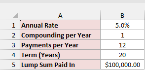
Enter this formula in B6 to get the matching monthly rate:
=(1+B1/B2)^(B2/B3)-1
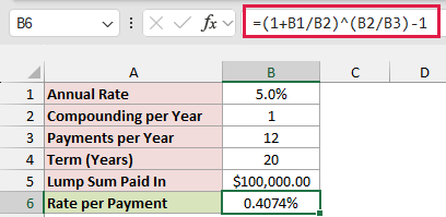
The monthly rate is 0.4074%, not the 0.4167% you get from 5%/12.
B1/B2 is the rate for each compounding period. Raising 1 plus that rate to B2/B3 converts it to the rate for each payment period.
Now use the converted rate in PMT. Enter this formula in B7:
=PMT(B6,B4*B3,-B5)
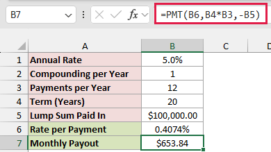
The payout is $653.84 a month, compared with $659.96 when the rate is simply divided by 12. That gap adds up to about $1,469 over 20 years.
If the rate compounds quarterly, change B2 to 4. The monthly rate becomes 0.4149% and the payout is $658.81.
For a rate that compounds once a year, the NOMINAL function gets you the same monthly rate: =NOMINAL(B1,B3)/B3 also returns 0.4074%.
Additional Notes About Calculating an Annuity in Excel
- Match the rate to the periods. =PMT(5%,240,-100000) uses an annual rate with monthly periods and returns $5,000.04 a month instead of $659.96.
- Give the lump sum and the payments opposite signs. With the same sign, RATE returns #NUM!, and NPER returns a meaningless negative number (-100.8 in the NPER example).
- NPER returns #NUM! when the payout is too small. $100,000 at 5% earns $416.67 a month, so a $400 payout never uses up the money.
- Set type to 1 when payments start today. Leaving it at 0 understates the lump sum in Method #2 by $1,262.71.
- These functions assume a fixed rate and equal payments. Fees, taxes, and payouts that rise with inflation need a more detailed model.
Frequently Asked Questions
Here are answers to a few common questions about annuity calculations in Excel.
How much does a $500,000 annuity pay per month?
At 5% a year for 20 years, =PMT(5%/12,240,-500000) returns $3,299.78 a month.
Real annuity quotes also depend on the insurer, your age, and whether the payouts last for life, so treat this as an estimate.
Is there an annuity function in Excel?
There’s no single ANNUITY function. PMT, PV, FV, NPER, and RATE are Excel’s annuity functions, and each one solves for a different unknown.
How do I calculate a growing annuity in Excel?
PMT, PV, and FV assume every payment is the same. When payments grow by a fixed percentage each year, use a growing annuity formula instead.
How do I see the annuity balance month by month?
Build a schedule with the IPMT and PPMT functions, which split each payment into interest and principal. The loan amortization schedule calculator shows the same breakdown.
Conclusion
In this article, I showed you how to calculate an annuity in Excel with PMT, PV, and FV, and how to handle an annuity due.
You also saw how to find the term with NPER and the rate with RATE, the math formula behind PV, and how to convert a rate that compounds differently.
I hope you found this article helpful.
Other Excel articles you may also like:
