
Converting currency in Excel lets you compare prices, budgets, and invoices in the same currency.
You need an exchange rate as well as the amount. Changing a dollar symbol to a euro symbol only changes how the number looks.
I’ll show you how to use a fixed rate, handle several currencies with a rate table, and retrieve current or historical rates.
Method #1: Multiplying by a Fixed Exchange Rate
For a single exchange rate, I recommend multiplying your amounts by a rate stored in its own cell. You can change that cell whenever you need another rate.
Below I have a dataset of 10 product orders on the Fixed Rate sheet, with USD prices in C2:C11 that I want to convert to euros.
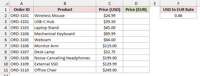
Column A contains Order IDs ORD-3101 through ORD-3110, and column B contains the products. F2 holds the manually entered USD-to-EUR rate, 0.86.
That means one US dollar buys 0.86 euros. You can get the rate you need from your bank or a currency website.
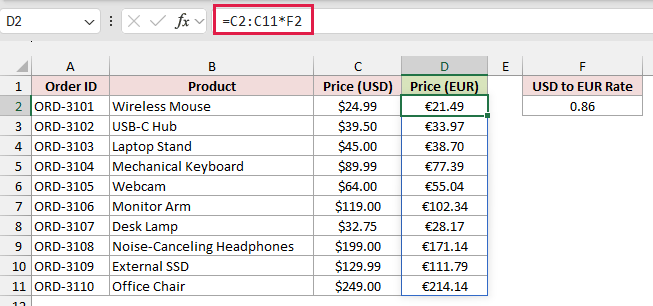
Enter this formula in D2:
=C2:C11*F2
How does this formula work?
The formula multiplies each USD price in C2:C11 by the rate in F2. In Excel with dynamic arrays, the results spill into D2:D11 automatically.
For example, the Wireless Mouse costs $24.99, which converts to €21.49. The Office Chair costs $249.00, which converts to €214.14.
Change F2, and every converted price updates. Keeping the rate in one cell saves you from editing the formula whenever the rate changes.
Column D uses a euro currency number format to display the results. The multiplication does the conversion; the format adds the symbol.
In older Excel, enter =C2*$F$2 in D2 and copy down; the absolute reference keeps the rate cell fixed.
Note: Check the direction of your rate. If it tells you how many dollars one euro buys, such as EUR to USD at 1.16, divide the USD amount by that rate instead.
Method #2: Using Paste Special (Convert in Place)
When you want to replace the original amounts, Paste Special can multiply them by a rate without leaving formulas behind.
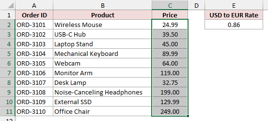
Below I have a dataset of 10 orders on the Paste Special sheet, with USD prices in C2:C11 that I want to replace with euro prices.
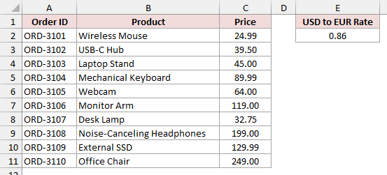
Columns A and B contain the Order IDs and products. Column C contains plain numbers with two decimal places, and E2 holds the USD-to-EUR rate, 0.86.
This method overwrites the USD prices. Work on a copy if you need to keep the originals.
Start by copying the exchange rate:
- Select E2 and press Ctrl + C.
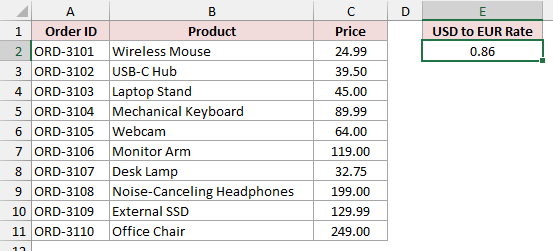
Next, select the prices you want to convert:
- Select C2:C11.
Set up Paste Special to multiply those prices:
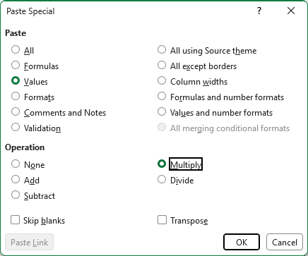
- On the Home tab, click Paste > Paste Special, or press Ctrl + Alt + V. Choose Values under Paste and Multiply under Operation.
Apply the conversion:
- Click OK.
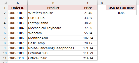
Column C now contains the euro prices. The first price becomes 21.49, and the last becomes 214.14.
Choosing Values preserves the prices’ existing number format instead of copying the rate cell’s format. Press Esc afterward to clear the copy selection.
These are fixed values. Changing E2 later won’t update them, so use Method #1 when you want the results to follow the rate.
Method #3: Using XLOOKUP With an Exchange Rate Table
When your amounts use several currencies, a lookup table lets each row use its own exchange rate.
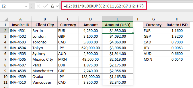
Below I have a dataset of 10 invoices on the Rate Table sheet, with amounts in six currencies that I want to convert to US dollars.
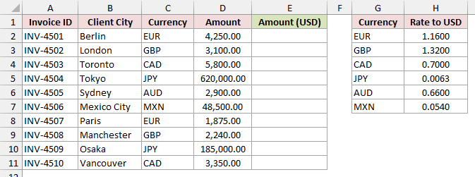
Columns A through D contain Invoice ID, Client City, Currency, and Amount. The Invoice IDs run from INV-4501 to INV-4510; column E will hold Amount (USD).
The rate table occupies G1:H7. Each sample rate represents US dollars per one unit of the currency: EUR 1.16, GBP 1.32, and CAD 0.70.
The remaining rates are JPY 0.0063, AUD 0.66, and MXN 0.054.
Enter this formula in E2:
=D2:D11*XLOOKUP(C2:C11,G2:G7,H2:H7)
How does this formula work?
XLOOKUP finds each currency code from C2:C11 in G2:G7. It returns the matching rate from H2:H7.
The formula then multiplies each amount in D2:D11 by its matching rate. The converted amounts spill into E2:E11 automatically.
For Berlin’s invoice, €4,250 multiplied by 1.16 returns $4,930.00. Tokyo’s ¥620,000 multiplied by 0.0063 returns $3,906.00.
If a currency code is missing from the rate table, XLOOKUP returns #N/A. Add the missing currency and its rate to the lookup ranges.
You can use this formula in Excel for Microsoft 365, Excel 2021, or Excel 2024.
In older Excel, enter =D2*VLOOKUP(C2,$G$2:$H$7,2,FALSE) in E2 and copy down; VLOOKUP finds the rate using an exact match.
Method #4: Using the Currencies Data Type (Live Rates)
For budgets that need current rates, Excel’s Currencies data type retrieves exchange-rate information online. This method requires Microsoft 365 or Excel for the web and an internet connection.
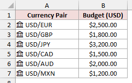
Below I have a dataset of six currency pairs and USD budgets on the Currencies Data Type sheet that I want to convert into local currencies.
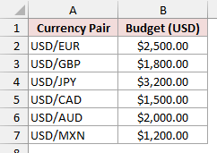
Column A contains USD/EUR, USD/GBP, USD/JPY, USD/CAD, USD/AUD, and USD/MXN as plain text in A2:A7.
The corresponding budgets in B2:B7 are $2,500, $1,800, $3,200, $1,500, $2,000, and $1,200. Type currency pairs as FROM/TO, using a slash.
Start by selecting the currency pairs:
- Select A2:A7.
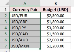
Convert the text into linked currency records:
- On the Data tab, click Data Types, then choose Currencies.
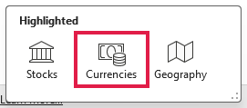
Excel converts each pair and displays a small building or bank icon beside it. The icons confirm that the cells now contain linked currency data.
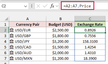
To retrieve the rates, enter this formula in C2 under Exchange Rate:
=A2:A7.Price
How does this formula work?
The .Price field returns the exchange rate for each linked pair. The formula spills into C2:C7; USD/EUR returns how many euros one dollar buys.
Now enter this formula in D2 under Local Budget:
=B2:B7*C2:C7
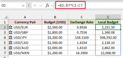
This formula multiplies each USD budget by its corresponding exchange rate. The local budgets spill into D2:D7 automatically.
The rates and converted amounts you see depend on when you refresh. Clicking a currency icon opens its card, which includes Name and Last trade time.
To update the rates and recalculate the budgets:
- On the Data tab, click Refresh All, or press Ctrl + Alt + F5.
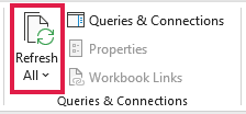
Refreshing these data types is manual unless you configure refresh settings. Right-click a currency cell and choose Data Type > Refresh Settings to adjust them.
Note: These rates can be delayed and don’t update tick by tick. They’re useful for budgeting, but you shouldn’t use them for trading decisions.
Method #5: Using STOCKHISTORY for Historical Rates
When the conversion needs an earlier date, STOCKHISTORY can retrieve the closing exchange rate for that day. You’ll need Microsoft 365 and an internet connection.
Below I have a dataset of eight euro invoices on the Historical Rates sheet that I want to convert to USD using their invoice dates.
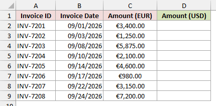
Column A contains Invoice IDs INV-7201 through INV-7208, column B contains Invoice Date, and column C contains Amount (EUR). Column D will hold Amount (USD).
The dates run from September 1 to September 24, 2026, and all are weekdays. The first invoice is €3,400; the last is €7,200.
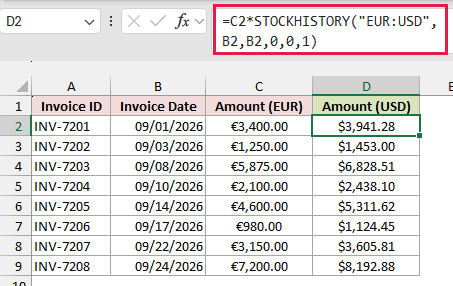
Enter this formula in D2, then copy it down to D9:
=C2*STOCKHISTORY("EUR:USD",B2,B2,0,0,1)
How does this formula work?
STOCKHISTORY retrieves historical rates as well as stock prices. Here, "EUR:USD" requests the euro-to-US-dollar pair using a colon.
The two B2 arguments set both the start and end date to the invoice date, so Excel requests one day’s rate.
The first 0 selects a daily interval. The second 0 removes headers, and 1 requests only the Close property.
That returns the closing rate, which the formula multiplies by the euro amount in C2. The September 1 invoice converts to $3,941.28.
After copying down, the September 24 invoice converts to $8,192.88.
This formula must be copied down. Passing B2:B9 as the date argument returns only one value; it doesn’t spill a separate result for every invoice date.
Cells can briefly display #BUSY! while Excel retrieves the data.
Note: A weekend or market-holiday date returns #VALUE!. Use =C2*TAKE(STOCKHISTORY("EUR:USD",B2-4,B2,0,0,1),-1) to search the preceding four days through the invoice date and take the last available closing rate on or before that date.
Additional Notes About Converting Currency in Excel
Whichever method you choose, keep these points in mind:
- Currency formatting changes the display, not the amount. Calculate the conversion before applying the destination currency’s symbol.
- Your bank’s exchange rate may include a markup. For accounting, use the rate your records actually require rather than assuming an online rate matches it.
- Use ROUND when an invoice requires amounts rounded to exact cents. Displaying two decimal places alone doesn’t round the stored result.
Here’s a quick comparison to help you choose a method:
| Method | Rate Source | Updates Automatically? | Excel Version |
|---|---|---|---|
| Fixed exchange rate | Manually entered rate | Results update when you edit the rate | All versions; use the copied-down formula in older Excel |
| Paste Special | Manually entered rate | No; converted values stay fixed | All versions |
| XLOOKUP rate table | Manually maintained table | Results update when you edit the table | Microsoft 365, 2021, 2024; use VLOOKUP in older Excel |
| Currencies data type | Online currency data | Manual refresh unless refresh settings are configured | Microsoft 365 or Excel for the web |
| STOCKHISTORY | Online historical closing rates | Retrieves rates for the specified dates | Microsoft 365 |
Frequently Asked Questions
Here are answers to a few other questions you may have about currency conversion in Excel.
Can I use Excel’s CONVERT function for currency?
No. CONVERT handles measurement units, such as miles, kilograms, and liters. It doesn’t convert money or retrieve exchange rates.
Can EUROCONVERT convert dollars to euros?
No. EUROCONVERT is available through the old Euro Currency Tools add-in and handles legacy euro-zone currencies. It isn’t useful for USD, GBP, or other currencies outside that group.
Why does my currency conversion formula show #SPILL!?
A spilling formula needs empty cells for its results. Data in that area can cause a #SPILL! error.
Move or clear the blocking data, then let Excel calculate again. For the fixed-rate example, D2:D11 must have room for all 10 results.
Conclusion
I recommend multiplying by a fixed exchange rate for most conversions because the rate is easy to check and change.
Use a rate table for several currencies, or choose the Currencies data type and STOCKHISTORY when you need current or historical rates.
Other Excel articles you may also like:
