
The DOLLAR function in Excel returns a number as currency-formatted text, rounded to the number of decimal places you choose.
It works well when currency must sit inside a sentence or label. For ordinary calculations, keep the value numeric and apply Currency or Accounting formatting.
In this article, I’ll show you how to control rounding, build readable labels, and avoid the text-result trap.
DOLLAR Function Syntax in Excel
Use DOLLAR with a number and an optional decimal-place setting:
=DOLLAR(number, [decimals])
- number (required) is the number, cell reference, or calculation you want to convert to currency text.
- decimals (optional) sets the digits after the decimal point. It defaults to 2, while a negative value rounds to the left of the decimal point.
When to Use DOLLAR Function
- Add standard currency formatting to numbers used inside sentences, labels, or report notes.
- Round currency text to whole dollars or broader place values.
- Show negative currency amounts in parentheses without building a custom format code.
- Create display-only report text that will not feed later calculations.
- Use Currency or Accounting cell formatting instead when the values must remain numeric.
Example 1: Convert Amounts to Currency Text
Let’s start with a column of billing adjustments.
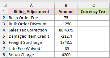
Below is the dataset. Column A names each adjustment, column B contains the raw amount, and the green Currency Text column will hold the formatted result.
We want one formula to format every amount as currency text.
Here is the formula:
=DOLLAR(B2:B8)
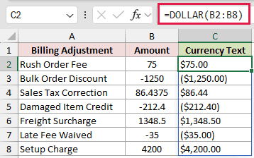
The formula returns $86.44 for Sales Tax Correction. Bulk Order Discount returns ($1,250.00), so negative amounts use parentheses.
This range formula spills in Excel 2021, Excel 2024, and Microsoft 365. In Excel 2019 and earlier, use a per-row version and fill it down.
If you need a fixed symbol or a minus sign instead of parentheses, TEXT offers more control. Currency or Accounting formatting keeps ordinary worksheet values numeric.
Example 2: Control Currency Rounding
Now let’s prepare rounded amounts for a renovation estimate.
Below is the dataset. Column A lists renovation items, column B holds the Contractor Estimate, and the empty green Whole Dollars and Nearest $100 columns will hold results.
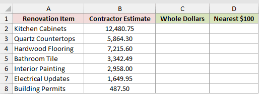
We want one view in whole dollars and another rounded to the nearest hundred.
Here is the whole-dollar formula:
=DOLLAR(B2:B8,0)
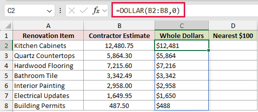
Setting decimals to 0 rounds each estimate to the nearest whole dollar. Kitchen Cabinets displays $12,481, while Building Permits displays $488.
Here is the formula for rounding to the nearest $100:
=DOLLAR(B2:B8,-2)
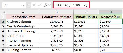
A negative decimals argument rounds to the left of the decimal point. Interior Painting becomes $3,000, while Electrical Updates becomes $1,600.
Example 3: Keep Currency in Reminder Text
Here’s where DOLLAR becomes especially useful.
Below is the dataset. Columns A and B hold customer names and balances. Column C will hold formatted reminders, while column D is the plain-joining comparison.
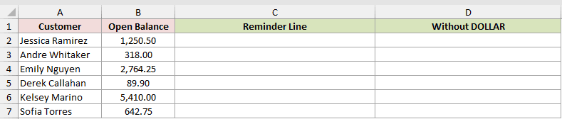
We want each reminder to keep the currency symbol, commas, and trailing zeros.
Here is the DOLLAR version:
=A2:A7&" has a balance of "&DOLLAR(B2:B7)
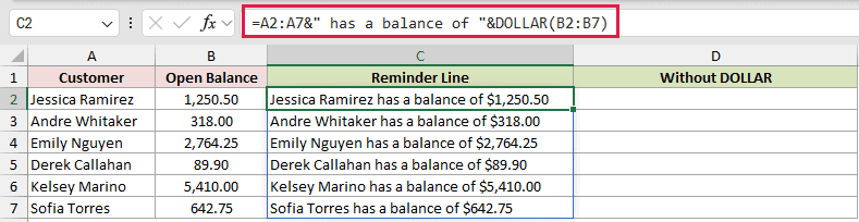
The first reminder reads Jessica Ramirez has a balance of $1,250.50. Andre Whitaker’s reminder reads Andre Whitaker has a balance of $318.00.
For comparison, this plain ampersand formula joins the raw balances, so the reminder loses its currency formatting:
=A2:A7&" has a balance of "&B2:B7
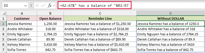
The comparison produces Jessica Ramirez has a balance of 1250.5 and Andre Whitaker has a balance of 318. The dollar signs and trailing zeros are gone.
Example 4: Format a Calculated Total
This example shows the main DOLLAR mistake.
Below is the dataset with stops, sales, and empty display text. A9:A10 are labeled SUM of Display Text and Formatted Total; B9 totals text by mistake, while B10 fixes it.
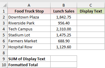
We want to see why formatted text cannot be totaled directly, then build the total from the source numbers.
First, here is the formula that converts each sale to display text:
=DOLLAR(B2:B7)
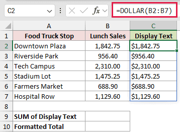
The displayed values include $1,842.75 for Downtown Plaza and $956.40 for Riverside Park. These results look numeric, but DOLLAR returns text.
This next formula is the mistake because it tries to total the text results:
=SUM(C2:C7)
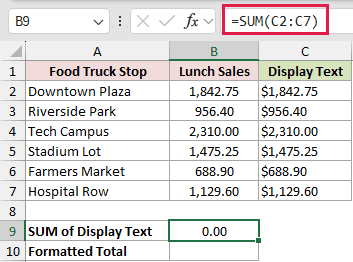
The mistake returns 0.00 because SUM skips the text in C2:C7.
The fix totals the numeric sales first, then applies DOLLAR to that result:
=DOLLAR(SUM(B2:B7))
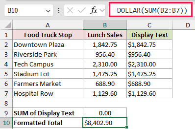
The corrected formula returns $8,402.90. Keep the arithmetic on the source numbers and convert only the final display value to text.
Example 5: Write Goal Progress Notes
Finally, let’s turn fundraising results into clear progress notes.
Below is the dataset. Column A lists team names, columns B and C hold Goal and Raised amounts, and the empty green Progress Note column will hold the notes.
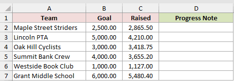
We want each note to state the direction and format the difference as currency.
Here is the formula:
=IF(C2:C7>=B2:B7,"Over goal by ","Under goal by ")&DOLLAR(ABS(C2:C7-B2:B7))
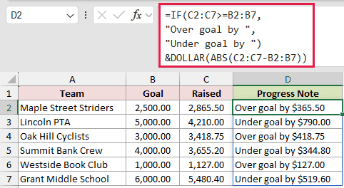
Maple Street Striders returns Over goal by $365.50. Lincoln PTA returns Under goal by $790.00.
IF chooses the wording, while ABS removes the sign before DOLLAR formats the difference. This avoids parentheses inside a sentence that already states the direction.
Tips & Common Mistakes
- DOLLAR returns text. Finish the arithmetic first, then use DOLLAR only for the value you want to display.
- The currency symbol follows your local language (regional) settings. Use TEXT when you need a fixed symbol or a different negative-number style.
- A truly blank input cell returns
$0.00, while nonnumeric text such asabcreturns#VALUE!. - VALUE can convert parentheses text such as
($89.50)back to a number, but keeping the original source values numeric is cleaner. - FIXED performs a similar text conversion without adding a currency symbol.
- The dollar sign in a cell reference, such as
$B$2, controls absolute referencing. It has nothing to do with the DOLLAR function.
Use the function when the finished wording matters as much as the amount itself.
The quickest warning sign is a currency value that looks right but refuses to behave like a number.
Other Excel articles you may also like:
